EPA Explained by Building It: Analyze Play-by-Play Data
What you'll build
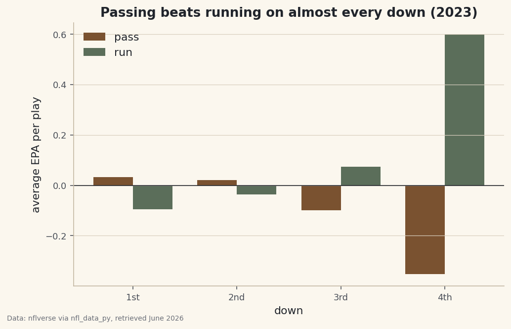
An EPA-per-play summary by down, computed straight from play-by-play.
If you read about NFL analytics for more than five minutes, you'll trip over three letters: EPA, Expected Points Added. It's the single most important number in the modern game, and yet most explanations either hand-wave it or bury it in math. Let's make it concrete with real per-play EPA from nflverse and put it to work on a question EPA was practically invented to settle: when does passing beat running? The answer turns out to be "almost always," and the data will show you exactly when and by how much.
This is an advanced tutorial in concept, though the code stays gentle - if you can group and average a DataFrame, you can do this. It builds directly on pulling your first NFL data, so I'll assume you've got the sdt_nflverse helper working and understand why we read nflverse's parquet files directly instead of fighting with nfl_data_py.
-
What EPA actually measures
Every game situation - down, distance, field position, time - has an expected points value: on average, how many points the team with the ball will eventually score from here. EPA is simply the change in that value caused by a single play. First-and-10 at your own 20 might be worth around one expected point; complete a 40-yard pass and the new situation is worth far more. The difference is that play's EPA. A positive EPA means the play helped your team's scoring outlook; a negative EPA means it hurt it.
That framing is powerful because it puts every play on one honest scale. A 4-yard run on 3rd-and-8 gains yards but loses expected points, because it failed to move the chains. A 9-yard completion on the same down is a big win. Raw yards can't see that distinction; EPA can. The beautiful part for us is that nflverse has already computed EPA for every play, so we don't have to build the expected-points model ourselves - we just have to use the column thoughtfully.
-
Load EPA and keep the real plays
We pull just the columns we need for one season, then filter down to ordinary pass and run plays that happened on a real down and carry an EPA value. Dropping the rows without a
downremoves kickoffs, extra points, and timeouts; dropping null EPA removes the handful of plays the model can't score.python import matplotlib.pyplot as plt import numpy as np import sdt_common as sdt import sdt_nflverse as nfl sdt.init("epa-explained-by-building-it") pbp = nfl.import_pbp_data([2023], columns=["posteam", "down", "play_type", "epa", "yardline_100"]) # Keep ordinary pass/run plays on a real down, with an EPA value. plays = pbp[(pbp["play_type"].isin(["pass", "run"])) & (pbp["down"].notna()) & (pbp["epa"].notna())].copy() plays["down"] = plays["down"].astype(int)The
.copy()after filtering is a small but important habit: it tells pandas we want a fresh DataFrame, not a view ontopbp, which keeps theSettingWithCopyWarningaway when we convertdownto an integer on the next line. -
Get a feel for the scale
Before averaging anything, let's see the range EPA lives on. We print the average across every play and the single best and worst plays of the season.
python with sdt.snippet("what-is-epa"): print("A positive EPA means the play helped; negative means it hurt.") print("Average EPA per play, 2023:", round(plays["epa"].mean(), 3)) print("\nBest and worst single plays this season:") print(" best :", round(plays["epa"].max(), 2), "EPA") print(" worst:", round(plays["epa"].min(), 2), "EPA")The scale of EPAA positive EPA means the play helped; negative means it hurt. Average EPA per play, 2023: -0.028 Best and worst single plays this season: best : 8.88 EPA worst: -12.44 EPA
Two things to absorb here. First, the league-wide average per play is negative - about -0.028. That's not a glitch: most plays nudge a team slightly backward relative to expectation, and offenses claw it back on the explosive plays. Second, look at the extremes. The best single play of the season was worth about +8.88 expected points (a defensive touchdown or a long score that flipped a desperate situation), and the worst was around -12.44 - the signature of a pick-six, where you not only fail to score but hand the other team seven. That ~21-point spread between the best and worst play is the canvas EPA paints on.
-
Average EPA by down and play type
Now the headline. We group by down and play type, take the mean EPA in each bucket, and reshape so passes and runs sit side by side for each down.
unstackpivots the play-type level out into columns;.loc[[1, 2, 3, 4]]just fixes the row order to 1st through 4th down.python # Average EPA by down and play type - the headline table. summary = (plays.groupby(["down", "play_type"])["epa"].mean() .unstack().round(3).loc[[1, 2, 3, 4]]) with sdt.snippet("epa-table"): print("Average EPA per play, by down:") print(summary.to_string())The table that explains modern NFL strategyAverage EPA per play, by down: play_type pass run down 1 0.032 -0.095 2 0.020 -0.037 3 -0.099 0.074 4 -0.352 0.598
Read this table slowly, because it contains most of what's driven a decade of play-calling change. On 1st and 2nd down, passing carries a clearly positive average EPA (about +0.032 and +0.020) while running is negative (-0.095 and -0.037). In other words, the "safe" early-down run is, on average, losing teams expected points. The gap is real and it is consistent.
Then look at the flip on later downs. On 3rd down the sign reverses - runs average +0.074, passes -0.099 - and on 4th down running is hugely positive (+0.598) versus passing's -0.352. This is a selection effect, not evidence that running is suddenly better. Teams only run on 3rd-and-4th down when it's short yardage they expect to convert; they're forced to pass on 3rd-and-long, the hardest situation in football. The play type is acting as a proxy for the distance to go.
-
Chart it: pass vs run on every down
Grouped bars make the early-down story jump out. We put one pair of bars per down - pass and run - and draw a line at zero so positive and negative EPA are visually unmistakable.
python # Grouped bars: pass vs run, for each down. downs = summary.index.astype(str) x = np.arange(len(downs)) w = 0.38 fig, ax = plt.subplots(figsize=(7.8, 4.8)) ax.bar(x - w / 2, summary["pass"], w, color=sdt.sport_color("football"), label="pass") ax.bar(x + w / 2, summary["run"], w, color=sdt.SPORT_COLORS["foundations"], label="run") ax.axhline(0, color="#20242B", linewidth=0.8) ax.set_xticks(x, ["1st", "2nd", "3rd", "4th"]) ax.set_xlabel("down") ax.set_ylabel("average EPA per play") ax.set_title("Passing beats running on almost every down (2023)") ax.legend(frameon=False) sdt.save_fig(fig, "epa_by_down", source="nflverse via nfl_data_py")Data: nflverse via nfl_data_py, retrieved June 2026 The
np.arangeand the±w/2offsets are the standard recipe for grouped bars: place each down at an integer position, then nudge the pass bar left and the run bar right by half a bar width so they sit shoulder to shoulder. The zero line drawn withaxhlineis what makes the chart legible - bars above it helped, bars below it hurt. On 1st and 2nd down the brown pass bars clear zero while the green run bars sink below it; that single visual is the case for early-down passing in one glance. -
Why passing usually wins - and the honest caveat
So why does passing beat running on the downs that matter most? Because incompletions cost less than they feel like they should (the down advances but field position rarely worsens), while completions routinely gain enough to flip expected points sharply upward. Runs, by contrast, are bounded: even a good 5-yard carry on 1st-and-10 usually fails to add expected points. The distribution of outcomes favors the pass.
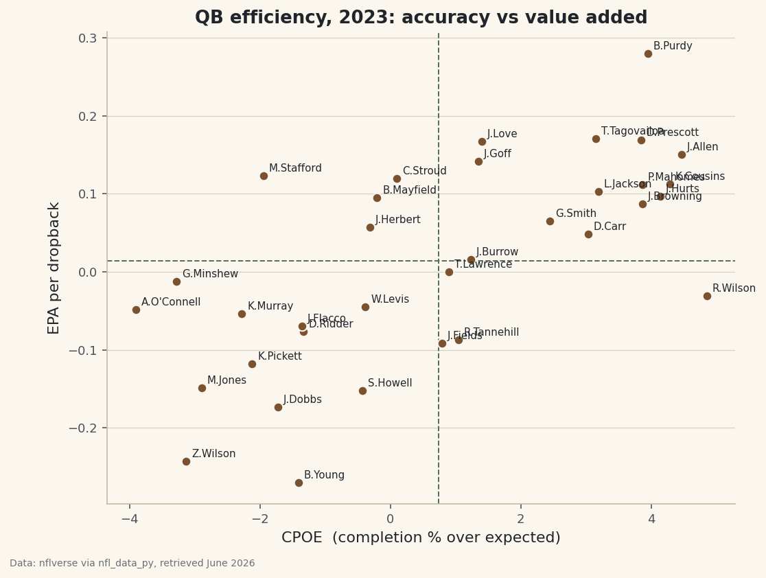
The honest caveat - and the reason a smart analyst never says "always pass" - is everything our averages hide. These numbers pool every team, defense, and game state together. A short-yardage run behind a dominant line, a kneel-down to end a half, the threat of the run that keeps the pass effective - none of that shows up in a marginal average. EPA tells you the league-wide tendency; it doesn't make a single play call for you. That distinction between population averages and individual decisions is worth carrying into the QB efficiency comparison, where we'll use a closely related metric, EPA per dropback, to rank passers.
Troubleshooting
AttributeError: 'DataFrame' object has no attribute 'append'
You're importing the real nfl_data_py on a modern pandas. It still calls the removed DataFrame.append() and crashes. Use the sdt_nflverse helper as the script does (it reads the same nflverse parquet with pandas.read_parquet), or set up a separate virtual environment pinned to pandas<2.0 / numpy<2.0 as described in the previous tutorial.
My EPA averages don't match - some are way off
You almost certainly left non-standard plays in the data. Kickoffs, two-point conversions, and penalties can carry extreme or null EPA. Make sure you filtered to play_type in {"pass", "run"}, dropped rows where down is null, and dropped null epa before grouping. A single un-filtered pick-six worth -12 EPA can drag a bucket's mean noticeably.
KeyError: 1 from .loc[[1, 2, 3, 4]]
This means down is still stored as a float (so the index is 1.0, not 1), or one down genuinely had no qualifying plays. Convert with plays["down"] = plays["down"].astype(int) after filtering out the null downs - casting before the dropna would error on the NaNs.
Challenge yourself
The 3rd and 4th down numbers are dominated by distance-to-go. Test that directly: add ydstogo to your column list, bucket 3rd-down plays into "short" (≤ 2 yards) and "long" (≥ 7 yards), and recompute average EPA by play type within each bucket. You should find that on 3rd-and-short the run advantage shrinks or flips, while on 3rd-and-long passing is the only option that isn't a disaster - proof that the play-type effect was really a distance effect in disguise.
Get the code
Here's the complete, working script for this tutorial. It runs exactly as shown.
Download the finished script (16_epa_explained_by_building_it.py)This script imports a small shared helper (and reads any bundled sample data) that live next to it in /downloads/ — grab these into the same folder so it runs as-is: sdt_common.py, sdt_nflverse.py.