Pull Your First NFL Data with nfl_data_py

Football might be the most data-rich sport in America, and nearly all of the public play-by-play traces back to one place: nflverse, a community project that quietly publishes every play of every game as free, tidy data files. It's a genuinely remarkable resource, and most people don't know it exists. We'll load a full 2023 season, glance at the schedule, and draw a pass-vs-run chart that shows at a glance which offenses lived through the air - finishing with a season of NFL data sitting in a DataFrame, ready for everything that comes after.

There's one wrinkle we need to deal with honestly up front. The library everyone reaches for, nfl_data_py, is broken on a modern Python install - and I'll show you exactly why, and a clean way around it. If you've already done the 12 essential pandas operations, every move here will feel familiar; this is just those same tools pointed at a bigger, more exciting dataset.

1. Understand the nfl_data_py problem first

   You'll find nfl_data_py in every tutorial and forum post about NFL data, so let's be clear about why we're not importing it directly. The library pins pandas<2.0 and numpy<2.0, and deep inside it still calls DataFrame.append() - a method pandas removed in version 2.0. On a current install it either refuses to install or, if you force it, crashes with AttributeError: 'DataFrame' object has no attribute 'append'. That's not your fault and it's not a bug in your code.

   Here's the key insight: under the hood, nfl_data_py isn't doing anything magical. It just downloads nflverse's public parquet files over HTTPS. So we can read those exact same files ourselves with one line of pandas and skip the broken dependency entirely. That's what our small sdt_nflverse helper does, and it deliberately copies nfl_data_py's function names so the code reads the same either way.

   If you're on a clean machine and would rather use the real library, the supported recipe is to make a fresh virtual environment pinned to the old pandas first, then install it:

   # OPTION A - the real library, in a fresh venv (needs old pandas)
   python -m venv nfl-env
   nfl-env\Scripts\activate          # Windows  (use: source nfl-env/bin/activate  on macOS/Linux)
   pip install "pandas<2.0" "numpy<2.0" nfl_data_py
   # then in your script:  import nfl_data_py as nfl

   We'll take Option B - read the parquet directly - because it works on any modern setup and teaches you what the library was doing all along.

2. Load a season of play-by-play, columns first

   Our helper exposes import_pbp_data, the same name nfl_data_py uses. The one habit worth forming immediately: pass a columns list. A full season of play-by-play has hundreds of columns and is roughly 20 MB on the wire; asking for only the seven we need makes the read noticeably quicker because parquet can pull just those columns off disk.

   import matplotlib.pyplot as plt
   
   import sdt_common as sdt
   import sdt_nflverse as nfl   # our drop-in; mirrors nfl_data_py's function names
   
   sdt.init("pull-your-first-nfl-data-with-nfl-data-py")
   
   # Pulling only the columns we need keeps the 20 MB file quick to read.
   pbp = nfl.import_pbp_data([2023], columns=[
       "game_id", "posteam", "play_type", "pass", "rush", "epa", "yards_gained"])

   Note that import_pbp_data takes a list of years, even for a single season - that's deliberate, so you can ask for several seasons at once later. posteam is the team with possession (the offense on that play), and epa is Expected Points Added, which we'll dig into in the next tutorial.

3. Check what you loaded

   Always look at your data before you trust it. We print the row count and show a handful of real plays. The sdt.show_df helper just prints the first few rows trimmed to fit a narrow column - nothing you couldn't do with .head().

   with sdt.snippet("shape"):
       print("Plays in the 2023 season:", f"{len(pbp):,}")
       sdt.show_df(pbp[["game_id", "posteam", "play_type", "yards_gained", "epa"]].dropna(), n=6)

   A full season, loaded

   Plays in the 2023 season: 49,665
              game_id posteam play_type  yards_gained       epa
   1  2023_01_ARI_WAS     WAS   kickoff           0.0  0.000000
   2  2023_01_ARI_WAS     WAS       run           3.0 -0.336103
   3  2023_01_ARI_WAS     WAS      pass           6.0  0.703308
   4  2023_01_ARI_WAS     WAS       run           2.0  0.469799
   5  2023_01_ARI_WAS     WAS      pass           0.0 -0.521544
   6  2023_01_ARI_WAS     WAS      pass          12.0  1.173155

   Just under 50,000 plays for the whole season - that's every snap, kickoff, and punt across all 272 regular-season and playoff games. Notice the game_id format: 2023_01_ARI_WAS reads as season, week, away team, home team. That single column tells you almost everything about when and where a play happened, and you'll lean on it constantly. The first row is a kickoff with an EPA of exactly 0, while the pass on the next line added about 0.70 expected points - your first taste of how EPA scores individual plays.

4. Pull the schedule

   Play-by-play tells you what happened inside games; the schedule tells you the games themselves - matchups, final scores, weeks. Our helper's import_schedules reads nflverse's one combined games file and filters to the season you ask for.

   schedule = nfl.import_schedules([2023])
   with sdt.snippet("schedule"):
       cols = ["week", "away_team", "away_score", "home_team", "home_score"]
       print("A few games from the schedule:")
       sdt.show_df(schedule[cols].dropna().tail(6), n=6)

   The tail of the 2023 schedule

   A few games from the schedule:
        week away_team  away_score home_team  home_score
   279    20        GB        21.0        SF        24.0
   280    20        TB        23.0       DET        31.0
   281    20        KC        27.0       BUF        24.0
   282    21        KC        17.0       BAL        10.0
   283    21       DET        31.0        SF        34.0
   284    22        SF        22.0        KC        25.0

   Because we took the tail, these are the last games of the season - and there it is: week 22, SF at KC, final score 25-22. That's Super Bowl LVIII. The schedule is the backbone of any standings or win-rate analysis, which is exactly how we'll use it in the capstone tutorial.

5. Count pass vs run plays by team

   Now a real question: how pass-happy is each offense? We keep only ordinary pass and run plays, then use pivot_table to count plays per team for each play type. Using aggfunc="size" counts rows, so the value column we pass doesn't matter much - we're tallying how many plays of each kind each team ran.

   # How pass-happy is each team? Count pass vs run plays by offense.
   plays = pbp[pbp["play_type"].isin(["pass", "run"])]
   by_team = plays.pivot_table(index="posteam", columns="play_type",
                               values="epa", aggfunc="size", fill_value=0)
   by_team["total"] = by_team["pass"] + by_team["run"]
   by_team = by_team.sort_values("total")

   Sorting by total puts the busiest offenses at the top of the chart (matplotlib draws horizontal bars from the bottom up). The fill_value=0 guards against any team-and-type combination that somehow had no plays, so we never get a stray NaN in the bars.

6. Draw the stacked bar chart

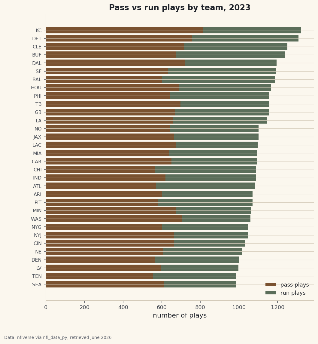
   A stacked horizontal bar is the right picture here: each team gets one bar, split into its pass portion and its run portion. We draw the pass plays first, then stack the run plays on top by setting left= to where the pass bar ended.

   fig, ax = plt.subplots(figsize=(8, 8.6))
   ax.barh(by_team.index, by_team["pass"], color=sdt.sport_color("football"), label="pass plays")
   ax.barh(by_team.index, by_team["run"], left=by_team["pass"],
           color=sdt.SPORT_COLORS["foundations"], label="run plays")
   ax.set_title("Pass vs run plays by team, 2023")
   ax.set_xlabel("number of plays")
   ax.tick_params(axis="y", labelsize=8)
   ax.legend(loc="lower right", fontsize=9, frameon=False)
   sdt.save_fig(fig, "pass_run_by_team", source="nflverse via nfl_data_py")

   

   The sdt.save_fig helper stamps every chart with its data source and the date it was retrieved - here, nflverse, retrieved June 2026 - so the provenance always travels with the image. Read the chart by comparing the length of each color: a long brown segment relative to the green means a pass-leaning offense. The bar lengths also reflect pace - teams that run more total plays (faster offenses, more overtime) reach further right regardless of their pass-run mix.

Troubleshooting