Same Question, Five Sports: Quantifying Home Advantage Across Leagues

This is the capstone, and it's the tutorial I'm proudest of, because it does the thing the whole site is secretly about: taking five separate skills you learned in isolation and pointing all of them at one question at the same time. The question is the oldest argument in any sports bar - how big is home advantage, really? Everybody has a feeling about it; almost nobody has a number. We'll get the number the honest way - the share of games actually won by the home team - across five leagues at once: MLB, the NBA, the Premier League, the NFL, and the NHL, all on one chart, caveats and all. And the answer is more interesting than "home teams win more," I promise.

What makes this a capstone isn't any one technique - it's that you'll reuse every data-access pattern the site taught, side by side in one script: a polite API session hitting two different sports endpoints, the nflverse parquet helper, a CSV read straight off the web, and a bundled fallback for the one source that blocks automated servers. It draws together the Statcast leaderboard, EPA explained by building it, and the NHL shot-location plot. If you've done those, you've already done the hard parts - today is about composition.

1. One question, five data sources

   The trick to a project like this is to give each league its own small function that returns the same shape: a home-win rate, a game count, and a season label. Once every source conforms to that contract, the rest of the program treats all five identically - even though each league forces a different access method.

   import io
   import os
   
   import matplotlib.pyplot as plt
   import pandas as pd
   
   import sdt_common as sdt
   import sdt_nflverse as nfl
   
   sdt.init("quantifying-home-advantage-across-five-leagues")
   HERE = os.path.dirname(os.path.abspath(__file__))
   session = sdt.polite_session()

   That single polite_session() - a requests session with real browser headers and automatic retry with backoff - is the same well-behaved client we've used for every live API on the site. We'll share it across the MLB, NHL, and soccer pulls.

2. MLB and NHL: two live APIs, one session

   Baseball and hockey both publish official standings that already carry each team's home record, so we never need to scan individual games. For MLB we read the Stats API standings and dig into each team's splitRecords for the "home" split. For the NHL we read the standings and sum the home wins, losses, and overtime losses across all teams.

   def mlb_home():  # MLB Stats API standings carry each team's home W-L split
       r = session.get("https://statsapi.mlb.com/api/v1/standings",
                       params={"leagueId": "103,104", "season": "2023",
                               "standingsTypes": "regularSeason"}, timeout=30).json()
       hw = hl = 0
       for grp in r["records"]:
           for tr in grp["teamRecords"]:
               for s in tr["records"]["splitRecords"]:
                   if s["type"] == "home":
                       hw += s["wins"]; hl += s["losses"]
       return hw / (hw + hl), hw + hl, "2023"
   
   def nhl_home():  # NHL standings carry home wins / losses / OT losses
       teams = session.get("https://api-web.nhle.com/v1/standings/now", timeout=30).json()["standings"]
       hw = sum(t["homeWins"] for t in teams)
       hl = sum(t["homeLosses"] for t in teams)
       ho = sum(t["homeOtLosses"] for t in teams)
       return hw / (hw + hl + ho), hw + hl + ho, "2024-25"

   Notice the small honesty in nhl_home: hockey has no ties, but it does have overtime/shootout losses, so the denominator is wins plus regulation losses plus OT losses. Get that wrong and the rate is subtly inflated. This is the same NHL API you met in the shot-location tutorial, just asking it a season-level question instead of a play-level one.

3. NFL: the nflverse helper, counting games

   For football we reuse the exact helper from the NFL tutorials. nflverse's schedule file has the final score of every game, so the home-win rate is just a comparison we average over all regular-season games.

   def nfl_home():  # nflverse schedules have the score of every game
       s = nfl.import_schedules([2023])
       g = s[(s["game_type"] == "REG")].dropna(subset=["home_score", "away_score"])
       return (g["home_score"] > g["away_score"]).mean(), len(g), "2023"

   The pattern (g["home_score"] > g["away_score"]).mean() is worth committing to memory: a comparison produces a column of True/False, and the mean of booleans is the fraction that are True - here, the home-win rate, in one line. Because we use sdt_nflverse, this works on a modern pandas; the real nfl_data_py would crash with the DataFrame.append() error covered in the EPA tutorial and its siblings.

4. Soccer: a CSV straight off the web

   The Premier League comes from football-data.co.uk, which publishes every season as a plain CSV. We download the bytes and read them directly into pandas without ever touching disk. The column we want is FTR - full-time result - coded H, D, or A for home win, draw, or away win.

   def soccer_home():  # football-data.co.uk: FTR = full-time result (H/D/A)
       raw = session.get("https://www.football-data.co.uk/mmz4281/2324/E0.csv", timeout=30).content
       df = pd.read_csv(io.BytesIO(raw)).dropna(subset=["FTR"])
       return (df["FTR"] == "H").mean(), len(df), "2023-24 EPL"

   Wrapping the downloaded bytes in io.BytesIO lets pd.read_csv treat them like a file - a tidy way to read a remote CSV in memory. Keep that FTR == "H" line in mind: it counts only home wins, and as we'll see, that "only" matters enormously for soccer.

5. NBA: an honest bundled fallback

   The NBA is the asterisk. Its stats endpoint, stats.nba.com, blocks automated build servers outright, so a live pull would simply fail when this site rebuilds. Rather than fake it or skip basketball, we bundle a CSV of the season's real game results and read that instead - clearly labeled so nobody mistakes it for a live figure.

   def nba_home():  # stats.nba.com blocks our build server, so we use the bundled real results
       d = pd.read_csv(os.path.join(HERE, "nba_home_results.csv"))
       return (d["home_pts"] > d["away_pts"]).mean(), len(d), "2023-24 (bundled)"

   This is a real lesson, not a cop-out. Sometimes the only thing that keeps an automated pipeline reliable is to cache real data and be transparent about it. The numbers are genuine 2023-24 results; only the delivery is local, and the "(bundled)" tag rides along to the final table so the provenance is never lost.

6. Assemble and rank the five leagues

   With five functions that all return the same triple, the orchestration is trivial. We map each league to its sport color and its function, call them in a loop, and build one DataFrame sorted by home-win rate.

   leagues = {"MLB": ("baseball", mlb_home), "NBA": ("basketball", nba_home),
              "EPL": ("soccer", soccer_home), "NFL": ("football", nfl_home),
              "NHL": ("hockey", nhl_home)}
   
   rows = []
   for name, (sport, fn) in leagues.items():
       pct, n, season = fn()
       rows.append({"League": name, "sport": sport, "HomeWin%": round(pct * 100, 1),
                    "Games": n, "Season": season})
   table = pd.DataFrame(rows).sort_values("HomeWin%", ascending=False).reset_index(drop=True)
   
   with sdt.snippet("table"):
       show = table.copy()
       show.index = range(1, len(show) + 1)
       print("Share of games won by the home team:")
       print(show.to_string())

   Home-win rate across five leagues

   Share of games won by the home team:
     League       sport  HomeWin%  Games             Season
   1    NFL    football      55.5    272               2023
   2    NBA  basketball      54.3   1231  2023-24 (bundled)
   3    NHL      hockey      52.2   1312            2024-25
   4    MLB    baseball      52.1   2430               2023
   5    EPL      soccer      46.1    380        2023-24 EPL

   There's the answer, ranked. The NFL has the biggest home edge - the home team won 55.5% of 272 games in 2023. The NBA is close behind at 54.3%, then the NHL at 52.2% and MLB at 52.1%, both barely above an even split. And the Premier League sits dead last at 46.1%. Each row uses that league's most recent complete season, which is why the seasons differ (the NHL figure is 2024-25; the NBA figure is the bundled 2023-24 real results), and every count is the real number of games measured.

7. Chart it - and read it honestly

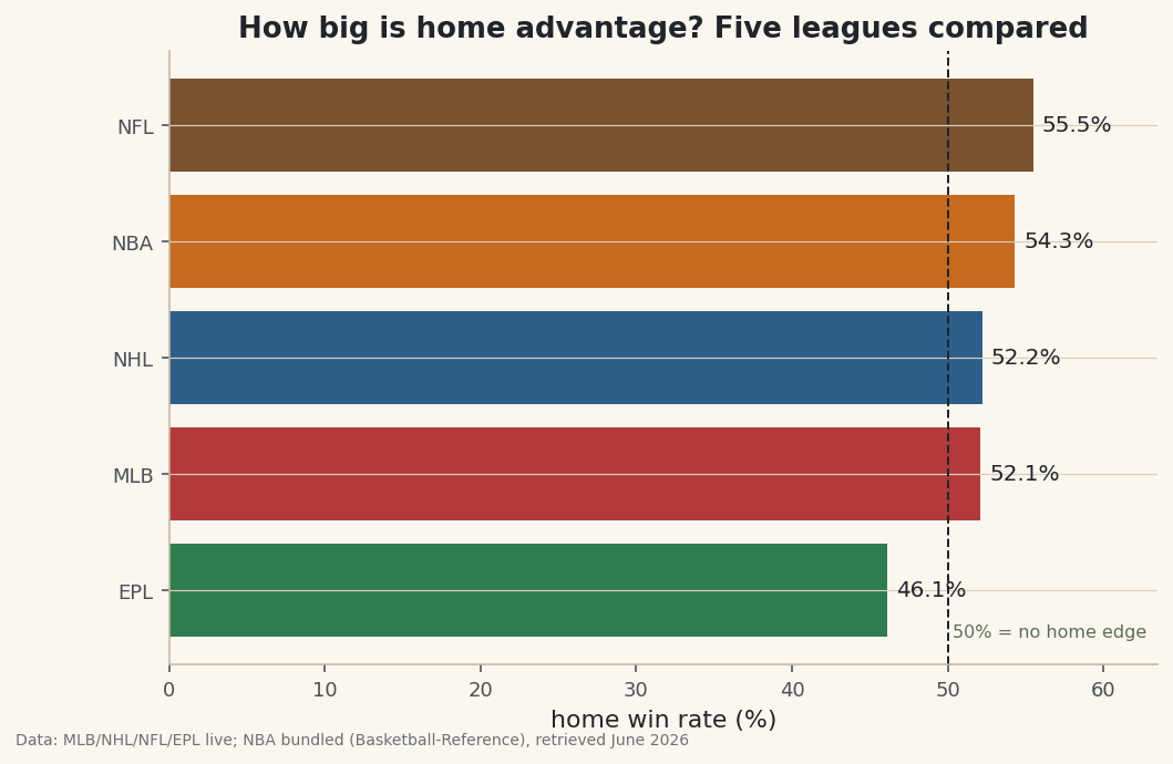
   A horizontal bar chart, colored by sport, with a dashed line at 50% to mark "no home edge at all," tells the story instantly. Anything left of that line means the home team won less than half its games.

   plot_df = table.sort_values("HomeWin%")
   colors = [sdt.SPORT_COLORS[s] for s in plot_df["sport"]]
   fig, ax = plt.subplots(figsize=(8, 5))
   bars = ax.barh(plot_df["League"], plot_df["HomeWin%"], color=colors)
   ax.bar_label(bars, fmt="%.1f%%", padding=4, fontsize=10)
   ax.axvline(50, color="#20242B", linestyle="--", linewidth=1)
   ax.text(50.3, -0.4, "50% = no home edge", fontsize=8, color=sdt.SPORT_COLORS["foundations"])
   ax.set_xlim(0, max(plot_df["HomeWin%"]) + 8)
   ax.set_xlabel("home win rate (%)")
   ax.set_title("How big is home advantage? Five leagues compared")
   sdt.save_fig(fig, "home_advantage",
                source="MLB/NHL/NFL/EPL live; NBA bundled (Basketball-Reference)")

   

   Now the crucial caveat, because a naive reading of this chart is wrong. The Premier League's 46.1% looks like soccer teams are worse at home - but that's an artifact of how we defined the metric. We counted home wins only, and soccer is the one sport here where a game can end in a draw. Roughly one in four EPL matches is a tie, and a draw isn't a home win, so it drags the rate down even when the home side genuinely held an edge. The other four leagues effectively have no draws, so nearly every game is forced into a win for somebody. We're not comparing five identical quantities; soccer's denominator includes a third outcome the others lack.

   Read correctly, the honest takeaways are: home advantage is real and positive in the four leagues that can't end in a draw, it's largest in the NFL, and the EPL's low win rate is mostly a draw effect rather than evidence that home soccer teams are disadvantaged. That distinction - between what a number literally measures and what it appears to say - is the most important habit in all of sports analytics, and a fitting note to end the site on.

Troubleshooting