I'll let you in on something that took me embarrassingly long to figure out: you don't need to know all of pandas. You need about twelve moves. Load a file, look at its shape, pick some columns, filter some rows, sort, group, join - that handful, recombined, is most of what I do in a real project. This page is those twelve, run one after another against the 2023 MLB standings (the final 30-team table, bundled as sample_standings.csv so it works completely offline). Every output you see below is the real thing the code printed on my machine.

Treat this one as a reference, not a read-once. I still keep it open in a tab and steal from it. It assumes you've already set up Python; the data is the 2023 regular-season standings I pulled from the MLB Stats API in June 2026 and saved next to the script.

Read a CSV and look at its shape (operations 1–2)

Everything starts with loading data. pd.read_csv turns a comma-separated file into a DataFrame — a table with named columns and numbered rows. The first thing I check on any new table is its .shape, a quick (rows, columns) sanity check that I loaded what I expected.

python

import pandas as pd

df = pd.read_csv("sample_standings.csv")
print("Shape (rows, columns):", df.shape)
print(df.head(5).to_string())

30 teams, 11 columns

Shape (rows, columns): (30, 11)
      Team Abbr League    Division    G    W   L  WinPct   RS   RA  RunDiff
0   Braves  ATL     NL     NL East  162  104  58   0.642  947  716      231
1  Orioles  BAL     AL     AL East  162  101  61   0.623  807  678      129
2  Dodgers  LAD     NL     NL West  162  100  62   0.617  906  699      207
3     Rays   TB     AL     AL East  162   99  63   0.611  860  665      195
4  Brewers  MIL     NL  NL Central  162   92  70   0.568  728  647       81

Thirty rows, eleven columns — one row per team, exactly right. The second operation is reading the column types with .dtypes, because pandas guesses a type for each column and you want to confirm the numbers came in as numbers, not text.

python

print(df.dtypes)

Output

Team            str
Abbr            str
League          str
Division        str
G             int64
W             int64
L             int64
WinPct      float64
RS            int64
RA            int64
RunDiff       int64
dtype: object

The text columns show as str and the counts as int64; WinPct is float64. If a column you expected to be numeric showed up as str, that's your signal something in the file needs cleaning — the whole subject of cleaning messy sports data.

Select columns and filter rows (operations 3–4)

You rarely want every column at once. Passing a list of column names inside square brackets — note the double brackets — gives you just those, in that order.
python
```
df[["Team", "W", "L", "RunDiff"]]
```
Four columns, first five rows
```
      Team    W   L  RunDiff
0   Braves  104  58      231
1  Orioles  101  61      129
2  Dodgers  100  62      207
3     Rays   99  63      195
4  Brewers   92  70       81
```
Filtering rows works differently: you write a condition that produces a column of True/False, then index the DataFrame with it. This "boolean mask" keeps only the rows where the condition is True. Here we keep teams with more wins than losses.
python
```
winners = df[df["W"] > df["L"]]
print("Teams with a winning record:", len(winners))
```
Output
```
Teams with a winning record: 17
      Team League    W   L
0   Braves     NL  104  58
1  Orioles     AL  101  61
2  Dodgers     NL  100  62
3     Rays     AL   99  63
4  Brewers     NL   92  70
```
Seventeen of the thirty teams finished above .500. The expression df["W"] > df["L"] compares the two columns row by row; wrapping it in df[...] selects the matching rows.
Sort, and add a computed column (operations 5–6)

sort_values reorders rows by a column. Pass ascending=False to put the biggest values on top — here, the best run differentials.
python
```
df.sort_values("RunDiff", ascending=False)[["Team", "RunDiff"]]
```
Best run differentials first
```
      Team  RunDiff
0   Braves      231
2  Dodgers      207
3     Rays      195
7  Rangers      165
5   Astros      129
```
Notice the row numbers on the left jump around (0, 2, 3, 7, 5) — sorting moves the rows but keeps each one's original index, a handy reminder that the index travels with the data. Operation six creates a brand-new column by assigning to a name that doesn't exist yet. We compute each team's Pythagorean win expectation, a classic estimate of deserved winning percentage from runs scored and allowed.
python
```
df["PythagPct"] = (df["RS"] ** 2 / (df["RS"] ** 2 + df["RA"] ** 2)).round(3)
df[["Team", "WinPct", "PythagPct"]]
```
Output
```
      Team  WinPct  PythagPct
0   Braves   0.642      0.636
1  Orioles   0.623      0.586
2  Dodgers   0.617      0.627
3     Rays   0.611      0.626
4  Brewers   0.568      0.559
```
Compare the two columns: the Orioles' actual .623 sits well above their .586 expectation, the hallmark of a team that won more one-run games than the run math predicts.
Group and aggregate, then count categories (operations 7–8)

Grouping is the most powerful move here. groupby("Division") splits the table into one bucket per division; chaining ["RunDiff"].mean() then collapses each bucket to a single average. We round and sort the result.
python
```
by_div = df.groupby("Division")["RunDiff"].mean().round(1).sort_values(ascending=False)
print(by_div.to_string())
```
Average run differential by division
```
Division
AL East       74.0
NL East       19.6
NL West        3.0
AL West       -7.2
NL Central   -13.8
AL Central   -75.6
```
The AL East averaged a +74.0 run differential while the AL Central sat at −75.6 — a vivid picture of an unbalanced league. Operation eight, value_counts, is the shortcut for "how many rows fall in each category," here confirming the 15-and-15 split between the two leagues.
python
```
print(df["League"].value_counts().to_string())
```
Output
```
League
NL    15
AL    15
```

Rename columns and describe the numbers (operations 9–10)

Source data rarely uses the column names you'd choose. rename takes a dictionary mapping old names to new ones and returns a fresh DataFrame — here making RS and RA human-readable.

python

renamed = df.rename(columns={"RS": "RunsScored", "RA": "RunsAllowed"})
print("New column names:", list(renamed.columns))

Output

New column names: ['Team', 'Abbr', 'League', 'Division', 'G', 'W', 'L', 'WinPct', 'RunsScored', 'RunsAllowed', 'RunDiff', 'PythagPct']

Operation ten, describe, is the one-line summary I reach for on any numeric data: count, mean, standard deviation, min, max, and quartiles, all at once.

python

print(df[["W", "L", "RS", "RA"]].describe().round(1).to_string())

Summary statistics

           W      L     RS     RA
count   30.0   30.0   30.0   30.0
mean    81.0   81.0  747.7  747.7
std     13.1   13.1   82.9   82.1
min     50.0   58.0  585.0  647.0
25%     75.2   72.2  680.0  697.2
50%     82.0   80.0  742.5  721.0
75%     89.8   86.8  792.8  813.2
max    104.0  112.0  947.0  957.0

Two nice gut-checks fall out of this: average wins land at exactly 81.0 (half of a 162-game schedule, as they must across a whole league), and the highest run total of the season was 947.

Take the top N, and join another table (operations 11–12)

When you only want the leaders, nlargest beats sorting-then-slicing because it says exactly what you mean: the five rows with the most wins.
python
```
df.nlargest(5, "W")[["Team", "W", "RunDiff"]]
```
Top five teams by wins
```
      Team    W  RunDiff
0   Braves  104      231
1  Orioles  101      129
2  Dodgers  100      207
3     Rays   99      195
4  Brewers   92       81
```
Finally, the twelfth operation joins two tables. Real analysis constantly needs to attach extra information — here, a region label for each division. We build a small lookup DataFrame and merge it on the shared Division column.
python
```
regions = pd.DataFrame({
    "Division": ["AL East", "AL Central", "AL West", "NL East", "NL Central", "NL West"],
    "Region": ["East", "Central", "West", "East", "Central", "West"],
})
joined = df.merge(regions, on="Division", how="left")
joined[["Team", "Division", "Region"]]
```
Output
```
      Team    Division   Region
0   Braves     NL East     East
1  Orioles     AL East     East
2  Dodgers     NL West     West
3     Rays     AL East     East
4  Brewers  NL Central  Central
```
The how="left" means "keep every row of the left table and attach a match where one exists," which is the join you'll want roughly nine times out of ten. This is the same merge that turns cryptic player IDs into names in the exit-velocity leaderboard.
Turn a groupby into a chart

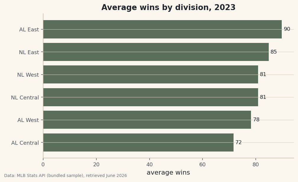
A summary is more persuasive as a picture. We reuse the grouping idea — average wins by division — and hand the result straight to matplotlib's horizontal bar chart. Sorting first makes the bars climb cleanly from bottom to top.
python
```
import matplotlib.pyplot as plt

wins = df.groupby("Division")["W"].mean().sort_values()
fig, ax = plt.subplots(figsize=(7.6, 4.4))
ax.barh(wins.index, wins.values)
ax.set_title("Average wins by division, 2023")
ax.set_xlabel("average wins")
ax.bar_label(ax.containers[0], fmt="%.0f", padding=3, fontsize=9)
fig.savefig("wins_by_division.png", dpi=144, bbox_inches="tight")
```
Data: Bundled sample (2023 MLB standings), retrieved June 2026

The same AL-East-on-top, AL-Central-at-the-bottom story from the run-differential numbers shows up instantly in bar length. That's the payoff of these twelve operations: a few lines take you from a raw CSV all the way to a finished, labeled chart.

Troubleshooting

FileNotFoundError when reading the CSV

pandas looked for sample_standings.csv relative to where you launched the script, not where the file lives. Either run the script from the folder that contains the CSV, or pass the full path. The downloadable script solves this by building an absolute path from its own location with os.path.dirname(os.path.abspath(__file__)).

KeyError: 'RunDiff'

pandas couldn't find a column by that exact name. Column names are case-sensitive and can carry stray spaces from the source file. Print list(df.columns) to see them exactly as loaded, and check for surprises like 'RunDiff ' with a trailing space — the kind of thing we fix in cleaning messy sports data.

SettingWithCopyWarning when adding a column

This appears when you assign to a column of a DataFrame that might be a slice of another one, so pandas can't tell if you meant to edit the original. If you filtered or selected before assigning, add .copy() at that step so you're clearly working on your own table, then add the column.

A numeric column behaves like text (string concatenation, not addition)

Run df.dtypes (operation 2). If a column shows str where you expected int64 or float64, a non-numeric character — a stray comma, a percent sign — forced it to text. Convert it with pd.to_numeric(df["col"], errors="coerce") after stripping the offending characters.

Challenge yourself

Combine several operations into one question: filter to the National League, group by division, and report the average run differential and the single best team by wins in each — then sort the result. For a stretch, join the Region lookup back on and produce average wins by region instead of by division. If you can chain those together cleanly, you've genuinely internalized these twelve moves.

Get the code

Here's the complete, working script for this tutorial. It runs exactly as shown.

This script imports a small shared helper (and reads any bundled sample data) that live next to it in /downloads/ — grab these into the same folder so it runs as-is: sdt_common.py, sample_standings.csv.

Pandas for Sports Data: The 12 Operations You'll Use Constantly

What you'll build

Read a CSV and look at its shape (operations 1–2)

Select columns and filter rows (operations 3–4)

Sort, and add a computed column (operations 5–6)

Group and aggregate, then count categories (operations 7–8)

Rename columns and describe the numbers (operations 9–10)

Take the top N, and join another table (operations 11–12)

Turn a groupby into a chart

Troubleshooting

Challenge yourself

Get the code

More Foundations tutorials

Setting Up Python for Sports Analytics: A Complete Beginner's Walkthrough

Your First Sports Data Visualization with matplotlib

Cleaning Messy Sports Data: Real-World Fixes for Real-World Files