Take any team's passes, place each player at their average position on the pitch, then draw a line between every pair who passed to each other - thicker for the pairs who combined most. What you get is a pass network: a kind of x-ray of a team's shape, of how it's built and which players hold it together. France in the 2018 World Cup final is my subject, from real StatsBomb event data, and the whole thing comes down to two aggregations - average positions and pass-pair counts - that every pass network is made of.

This builds on your first StatsBomb pull, so you already know how to load a match's events. This is an Advanced tutorial because we juggle two grouped views of the same data at once and join them on the chart - but every individual step is something you've seen before.

Attribution, as always: StatsBomb Open Data is free, but its license requires credit on anything you publish. We bake it into the figure and I'll remind you at the end. Data retrieved June 2026.

Load the match and choose a cutoff

We load the final and pick France (the home team) as our subject. Here's the convention that makes a pass network meaningful: we build it from passes before the first substitution. Once a team makes a change, the average positions blur together two different players in one spot, so freezing the network at the first sub keeps it a clean portrait of the starting eleven. We find the minute of the earliest substitution, defaulting to 200 (i.e. never) if there wasn't one.
python
```
import matplotlib.pyplot as plt
from mplsoccer import Pitch
from statsbombpy import sb

matches = sb.matches(competition_id=43, season_id=3)
final = matches[matches["competition_stage"] == "Final"].iloc[0]
TEAM = final["home_team"]
events = sb.events(int(final["match_id"]))

team_ev = events[events["team"] == TEAM]
subs = team_ev[team_ev["type"] == "Substitution"]
first_sub = subs["minute"].min() if len(subs) else 200
```
Storing the side in a TEAM variable instead of hard-coding "France" means one edit redraws the whole network for Croatia later. The first_sub minute is the gate everything downstream passes through.
Keep only completed passes before that cutoff

We now filter to the passes that build the network: France's passes, only the completed ones, and only those before first_sub. Remember the StatsBomb convention from the pass map - a successful pass has a blank pass_outcome, so completed means pass_outcome is NaN. We also drop any pass missing its location or its pass_recipient, since we need both to draw a line between two players.
python
```
passes = team_ev[(team_ev["type"] == "Pass")
                 & (team_ev["pass_outcome"].isna())
                 & (team_ev["minute"] < first_sub)].dropna(
                     subset=["location", "pass_recipient"]).copy()
passes["x"] = passes["location"].str[0]
passes["y"] = passes["location"].str[1]
```
The pass_recipient column names the team-mate who received each pass - that's the second half of every connection in the network. We pull x and y out of the location list as usual, because we'll average those positions in a moment.
Compute average positions and pass combinations

This is the conceptual core - two different groupings of the same passes. First, the nodes: group by player and take the mean of x and y to get each player's average position, then attach how many passes they made with value_counts(). Second, the edges: group by the pair (player, pass_recipient) and count how many times each combination occurred, keeping only pairs who connected at least three times so the chart isn't cluttered with one-off passes.
python
```
positions = passes.groupby("player")[["x", "y"]].mean()
positions["passes"] = passes["player"].value_counts()
combos = (passes.groupby(["player", "pass_recipient"]).size()
          .reset_index(name="n").query("n >= 3"))
```
Grouping by a list of two columns is the trick that turns individual passes into pair counts - .size() then tallies how many rows fell into each pair. The positions table is your nodes (where each player sat and how busy they were); combos is your edges (who linked with whom, and how often).
Check the busiest links

Let's confirm the pipeline by printing how many passes survived the cutoff and the most frequent combinations.
python
```
print(f"{TEAM}: {len(passes)} completed passes before the first substitution")
print("\nMost frequent passing combinations:")
print(combos.sort_values("n", ascending=False).head(6).to_string(index=False))
```
France's most frequent passing combinations
```
France: 111 completed passes before the first substitution

Most frequent passing combinations:
            player     pass_recipient  n
       Hugo Lloris     Olivier Giroud  7
   Benjamin Pavard     Raphaël Varane  4
        Paul Pogba    Benjamin Pavard  4
    Raphaël Varane Samuel Yves Umtiti  4
    Blaise Matuidi      N''Golo Kanté  3
Lucas Hernández Pi      N''Golo Kanté  3
```
France completed 111 passes before their first change, and the top link is goalkeeper Hugo Lloris to striker Olivier Giroud, seven times - the long clearances up to the target man, a real and recognisable pattern from that final. Behind it sit the defensive combinations that knit a back line together: Pavard–Varane, Pogba–Pavard, Varane–Umtiti, each connecting four times. You may notice the names look unusually formal and a couple are awkwardly cut, like Lucas Hernández Pi, and an apostrophe is doubled in N''Golo Kanté - that's the raw StatsBomb data, which stores full legal names and the odd escaping artifact. We'll shorten them for the chart next.

Draw the edges, then the nodes

We draw the pitch as always, then plot the network in two passes. First the edges: for each combination we look up both players' average positions and draw a line between them, its width scaled by how often they connected (n * 0.5), so heavily-used links are visibly thicker. Then the nodes on top: one marker per player at their average position, sized by how many passes they played (passes * 14 + 90).
python
```
pitch = Pitch(pitch_type="statsbomb", line_color="#20242B",
              pitch_color="#FBF7EE", linewidth=1.1)
fig, ax = pitch.draw(figsize=(8.6, 5.6))
fig.set_facecolor("#FBF7EE")

for _, r in combos.iterrows():
    if r["player"] in positions.index and r["pass_recipient"] in positions.index:
        a, b = positions.loc[r["player"]], positions.loc[r["pass_recipient"]]
        ax.plot([a["x"], b["x"]], [a["y"], b["y"]], color="#2E7D4F",
                linewidth=r["n"] * 0.5, alpha=0.5, zorder=1)

pitch.scatter(positions["x"], positions["y"],
              s=positions["passes"] * 14 + 90, ax=ax, color="#2E7D4F",
              edgecolor="#20242B", linewidth=1, zorder=3)
```
Order and zorder matter here: edges first at zorder=1 so the lines sit underneath, nodes at zorder=3 so the player dots are drawn cleanly on top of the web. The if guard skips any combo whose players somehow aren't in the positions table, which keeps the loop from erroring on an edge case.
Label the players with short names

Those full legal names would swamp the chart, so we write a tiny helper that returns a recognisable short name. StatsBomb's full names usually put the familiar surname second - "Kylian Mbappe Lottin" is stored in full, and the second word, "Mbappe", is the one fans know - so we split on spaces and take the second word, falling back to the first if there's only one. Then we drop a label just below each node.
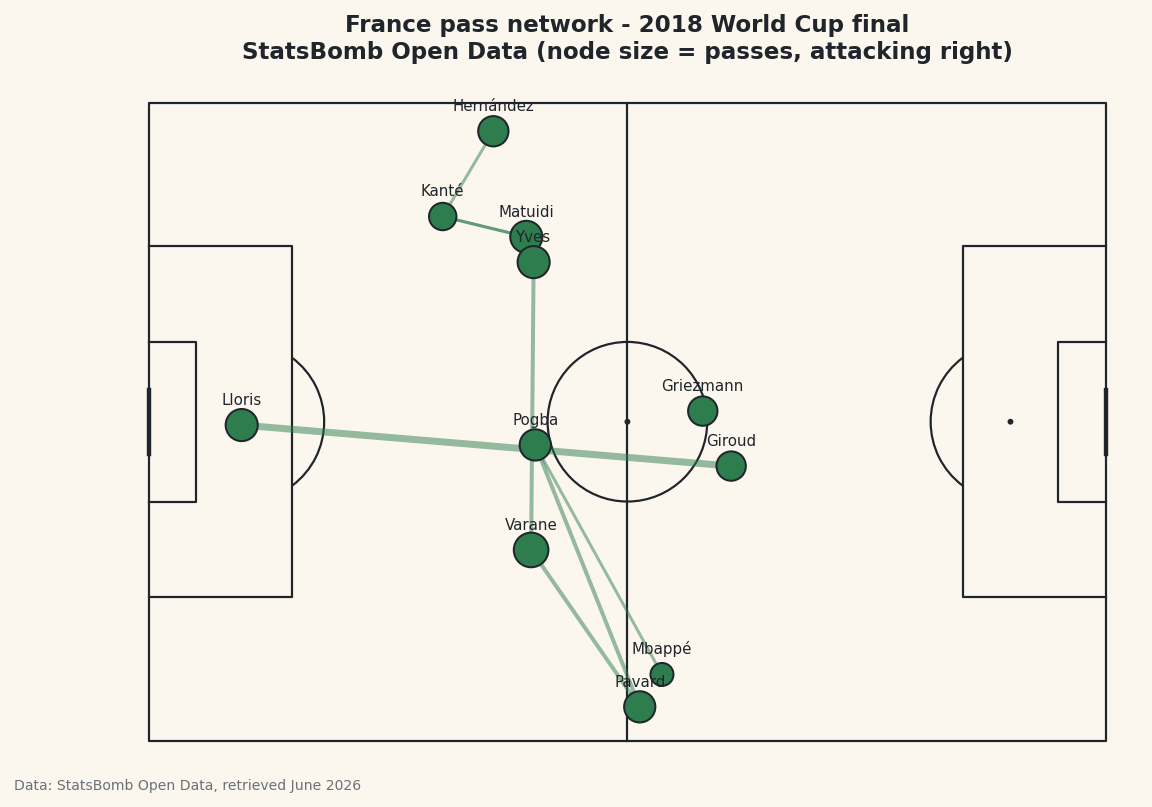
python
```
def short_name(full):
    parts = full.split()
    return parts[1] if len(parts) >= 2 else parts[0]

for player, r in positions.iterrows():
    ax.text(r["x"], r["y"] - 2.6, short_name(player), ha="center",
            fontsize=7.5, color="#20242B", zorder=4)
ax.set_title(f"{TEAM} pass network - 2018 World Cup final\n"
             f"StatsBomb Open Data (node size = passes, attacking right)",
             fontsize=11.5, color="#20242B")
fig.savefig("pass_network.png", dpi=144, bbox_inches="tight")
```
Data: StatsBomb Open Data, retrieved June 2026

The short_name heuristic isn't perfect - "Samuel Yves Umtiti" becomes "Yves" - so for a polished graphic you'd hand-correct the odd one. Read the finished network and France's structure jumps out: the big, central, heavily-linked nodes are the players the team ran through, and the thick line to Giroud up front shows their route to goal. The caption credits StatsBomb Open Data - required by the license every time you publish a chart from it.

Troubleshooting

The network is nearly empty or has too few lines

Two likely causes. You may have filtered pass_outcome the wrong way - completed passes have a blank outcome, so keep the .isna() rows. Or your n >= 3 threshold is too strict for a low-passing match; lower it to n >= 2 to see more links. Also confirm first_sub isn't tiny - an early substitution leaves very few passes.

KeyError when looking up a player in positions

A pass recipient who never made a pass themselves won't appear in positions (which is grouped by passer). That's exactly why the loop has the if r["player"] in positions.index and ... guard - keep it. If you removed it, add it back so missing players are skipped rather than crashing the draw.

The player labels are wrong or cut off

StatsBomb stores full legal names, so the short_name "take the second word" rule occasionally picks a middle name (e.g. "Yves" for Samuel Yves Umtiti). It's a heuristic, not a lookup. For a publication-grade chart, build a small dictionary mapping full names to display names and use that instead.

Challenge yourself

Color each node by pitch zone - defenders, midfielders, forwards - by binning the average x position into thirds, so the team's lines of shape read at a glance. Then make the edges directional: right now an A→B pass and a B→A pass are counted separately in combos, so try summing both directions to get the total volume between each pair, and see which partnership tops the list. For a real stretch, draw Croatia's network beside France's with one change to TEAM and compare how the two finalists were built - the same locations also drive the player heatmap.

Get the code

Here's the complete, working script for this tutorial. It runs exactly as shown.

This script imports a small shared helper (and reads any bundled sample data) that live next to it in /downloads/ — grab these into the same folder so it runs as-is: sdt_common.py.

Build a Team Pass Network

What you'll build

Load the match and choose a cutoff

Keep only completed passes before that cutoff

Compute average positions and pass combinations

Check the busiest links

Draw the edges, then the nodes

Label the players with short names

Troubleshooting

Challenge yourself

Get the code

More Soccer tutorials

Pull Your First Match Data with StatsBomb Open Data

Build an xG League Table from Understat Data

Draw a Pass Map with mplsoccer