Expected vs Actual: Find the Hitters Getting Unlucky
What you'll build
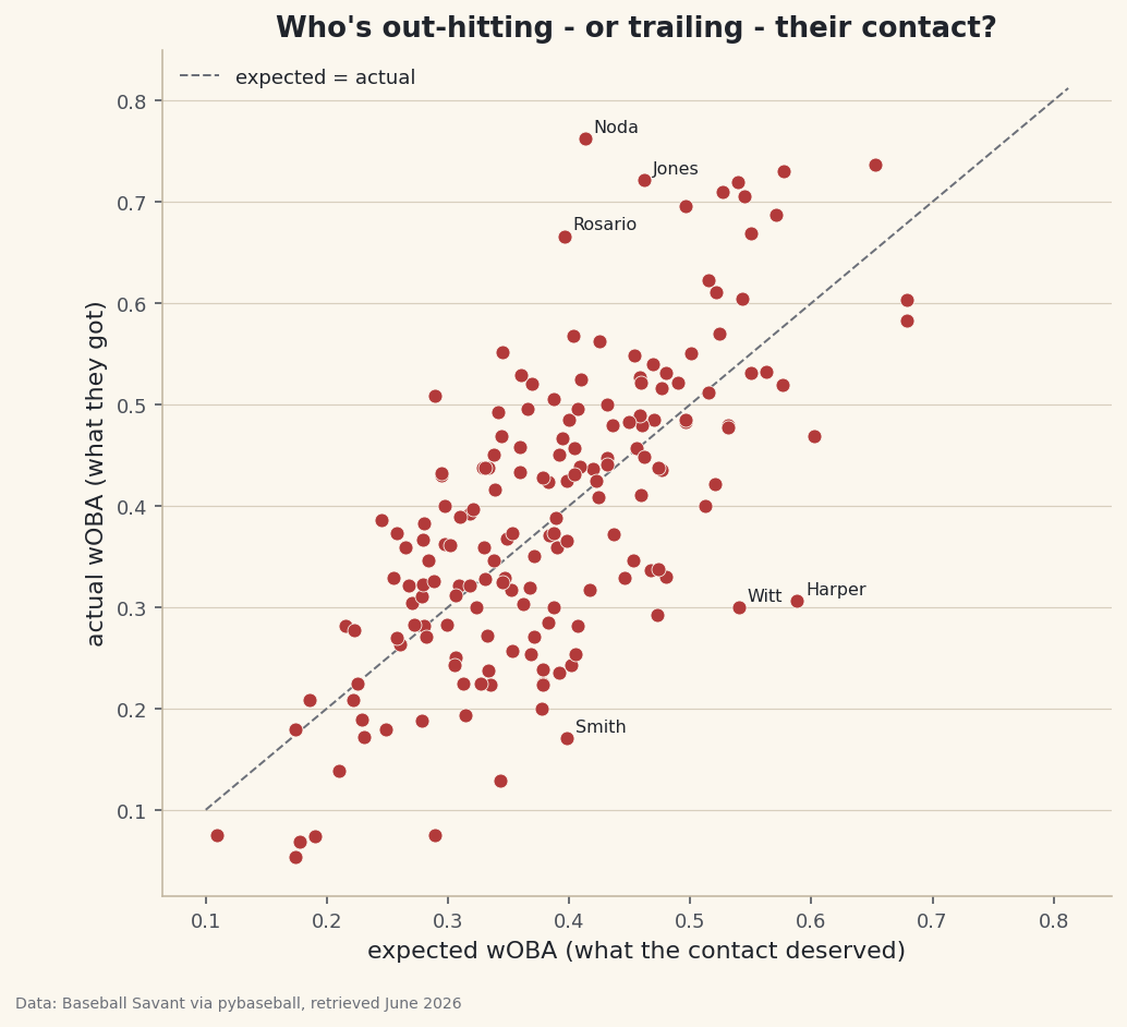
A chart of hitters whose results trail what their contact deserved.
Here's a hard truth that separates good analysts from box-score readers: a hitter can do everything right and still come up empty. Scald a line drive straight at the shortstop and the scoreboard says "out" - identical to a weak pop-up. Over a week or a month those bad bounces pile up, and the batting average lies about how well someone actually hit. We're going to catch that lie in the act — comparing what each hitter's contact deserved against what it actually produced, using Statcast's expected-stats model. The gap between the two is a clean, defensible measure of luck.
This is an advanced step, and it builds straight on the Statcast exit-velocity leaderboard - same week of data, same groupby-and-agg backbone, same player-ID lookup. If you've run that one, this week is already cached and the pull is instant. The data is Baseball Savant via pybaseball, retrieved June 2026.
-
The two numbers, and why they're the right two
We compare two flavors of wOBA (weighted On-Base Average), a one-number hitting metric scaled so that roughly .320 is league average and .400 is excellent. Actual wOBA is what happened - the credit a hitter earned from his real outcomes. Expected wOBA (xwOBA) is what Statcast's model says those same batted balls should have produced, based only on each ball's exit velocity and launch angle, ignoring where the fielders happened to be standing.
The logic is simple and powerful: launch speed and angle are things the hitter controls; defensive positioning and lucky bounces are not. So if a hitter's actual wOBA sits far below his expected wOBA, he hit the ball well but the results didn't follow - he's been unlucky and is a good bet to improve. If actual sits far above expected, he's been getting away with weak contact. The gap is the luck.
-
Pull the cached week and keep batted balls
We reuse the exact week from the leaderboard tutorial - the first week of June 2023 - so nothing new downloads. Then we keep only balls in play that have both an expected and an actual wOBA recorded.
python import matplotlib.pyplot as plt import pybaseball as pyb pyb.cache.enable() data = pyb.statcast("2023-06-01", "2023-06-07") bb = data[(data["type"] == "X")].dropna( subset=["estimated_woba_using_speedangle", "woba_value"]).copy()The column
estimated_woba_using_speedangleis Statcast's xwOBA for each batted ball - the model's verdict on what that contact deserved - andwoba_valueis the actual wOBA credit the play earned. We filter totype == "X"(in play) and drop rows missing either value, because we can't compute a gap without both. As always,.copy()on the slice avoids theSettingWithCopyWarningwhen we add a column next. -
Aggregate to one row per hitter
This is the familiar leaderboard move, now computing two averages side by side. We group by
batter, count each hitter's batted balls, and take the mean of both the actual and expected wOBA. Then we require a real sample so a single ball can't dominate.python MIN_BBE = 12 board = (bb.groupby("batter") .agg(bbe=("woba_value", "size"), actual=("woba_value", "mean"), expected=("estimated_woba_using_speedangle", "mean")) .query("bbe >= @MIN_BBE"))The named aggregations build all three columns in one pass:
bbecounts the batted balls,actualandexpectedaverage the two wOBA flavors. The@MIN_BBEinsidequerypulls in our Python variable so the threshold lives in one place - and over a single week, twelve batted balls is already a generous bar; lower it and the list fills with hitters whose averages swing wildly on one or two plays. -
Compute the luck gap
The whole tutorial comes down to one subtraction. Luck is actual minus expected: positive means a hitter out-performed his contact (fortunate), negative means his results trailed his contact (unlucky).
python board["luck"] = (board["actual"] - board["expected"]).round(3) board = board.round({"actual": 3, "expected": 3})We round everything to three decimals because wOBA lives on a .000-to-1.000ish scale where the third place is meaningful. That single
actual - expectedcolumn is the entire signal we set out to build; everything after this is turning IDs into names and drawing the picture. -
Turn IDs into names and find the extremes
Statcast gives us batter IDs, so we reverse-look-up the whole index at once and merge the names back on. Then we sort by the absolute size of the luck gap to surface the most extreme stories in either direction.
python names = pyb.playerid_reverse_lookup(board.index.tolist(), key_type="mlbam") names["player"] = names["name_first"].str.title() + " " + names["name_last"].str.title() board = board.merge(names.set_index("key_mlbam")["player"], left_index=True, right_index=True) extreme = board.reindex(board["luck"].abs().sort_values(ascending=False).index).head(8) print("Biggest gaps between results and contact quality (June 1-7, 2023):") print(extreme[["player", "bbe", "expected", "actual", "luck"]].to_string(index=False))The biggest luck gaps that weekBiggest gaps between results and contact quality (June 1-7, 2023): player bbe expected actual luck Ryan Noda 13 0.413 0.762 0.349 Bryce Harper 17 0.588 0.306 -0.283 Eddie Rosario 16 0.396 0.666 0.269 Nolan Jones 12 0.462 0.721 0.259 Bobby Witt 21 0.54 0.3 -0.24 Pavin Smith 17 0.398 0.171 -0.228 Ha-Seong Kim 12 0.289 0.508 0.219 Jake Mccarthy 14 0.343 0.129 -0.215The pattern to learn is
board["luck"].abs().sort_values(ascending=False).index: we sort by the magnitude of luck, grab that ordering as an index, andreindexthe board onto it so the most extreme hitters - lucky or unlucky - rise to the top together. The results read true: Ryan Noda's .762 actual wOBA towers over his .413 expected for a +0.349 gap - he got hits on contact that usually doesn't reward you. At the other pole, Bryce Harper crushed the ball (a .588 expected wOBA, elite contact) but managed only a .306 actual - a -0.283 gap, the unluckiest line on the board and a near-certain bet to bounce back. -
Plot expected against actual
The right chart for "predicted vs realized" is a scatter with a diagonal reference line where the two are equal. Every hitter is a dot; the dashed line is
expected = actual. Points above the line out-hit their contact; points below it are the unlucky ones whose results trailed what they earned.python fig, ax = plt.subplots(figsize=(7.8, 7)) ax.scatter(board["expected"], board["actual"], s=42, color="#B23A3A", edgecolor="#FBF7EE", linewidth=0.4, zorder=3) lo, hi = 0.1, board[["expected", "actual"]].values.max() + 0.05 ax.plot([lo, hi], [lo, hi], color="#6C7079", linestyle="--", linewidth=1, label="expected = actual") for _, r in board.reindex(board["luck"].abs().sort_values(ascending=False).index).head(6).iterrows(): ax.annotate(r["player"].split()[-1], (r["expected"], r["actual"]), fontsize=8, xytext=(4, 3), textcoords="offset points") ax.set_xlabel("expected wOBA (what the contact deserved)") ax.set_ylabel("actual wOBA (what they got)") ax.set_title("Who's out-hitting - or trailing - their contact?") ax.legend(frameon=False, fontsize=9) fig.savefig("xwoba_vs_woba.png", dpi=144, bbox_inches="tight")Data: Baseball Savant via pybaseball, retrieved June 2026 The diagonal is the trick that makes this readable. Drawing the line from
lotohi- the same range on both axes - means any dot's vertical distance from the line is its luck, no arithmetic required. We label only the six most extreme hitters withannotate, usingr["player"].split()[-1]to print just the last name and anxytextoffset to nudge it clear of the dot. Harper sits well below the line; Noda well above. Settingzorder=3keeps the dots drawn on top of the reference line. -
Read it like an analyst
The instinct to fight is treating one week's gap as a verdict on a hitter's talent - it isn't. Over seven days even an excellent
MIN_BBEsample is small, and luck is, by definition, noisy. What the chart genuinely earns you is a shortlist: the hitters whose underlying contact and surface results have pulled apart, which is exactly where reversion tends to happen next. A pro would read Harper's dot as "buy" and Noda's as "don't expect this to last," then widen the window to a month before betting anything real on it. That discipline - trusting the process metric over the small-sample result - is the whole reason expected stats exist.
Troubleshooting
KeyError: 'estimated_woba_using_speedangle'
That's the exact Statcast column name for xwOBA - check the spelling, including the underscores and the using_speedangle suffix. If pybaseball returned an older or trimmed schema, print data.columns.tolist() to confirm the column is present; on a normal statcast() pull it always is.
The same names from the leaderboard don't appear here
That's expected, and instructive. The exit-velocity leaderboard ranks by how hard hitters hit the ball; this ranks by the gap between deserved and actual results. A hitter can sit mid-pack in raw exit velocity yet top the luck list - they're measuring different things. Both lean on the same week, so you can join them on batter and explore the overlap.
The luck values look tiny - around 0.05
For most hitters that's correct: over a full season expected and actual wOBA nearly converge, which is the whole point of the metric. The eye-catching gaps live in small samples like our one week, where a couple of bad bounces move a hitter's actual wOBA a lot. Sort by luck.abs() as we do to pull the meaningful extremes to the top instead of scanning a wall of near-zeros.
The diagonal line doesn't reach the corner dots
The line runs from lo to hi, and hi is derived from the maximum of the data plus a small pad. If a single extreme actual wOBA sits outside that range, widen the pad (try + 0.08) or set lo/hi by hand so the reference line spans every point. A diagonal that stops short just means your data ran past the line's endpoints.
Challenge yourself
Turn this from a snapshot into a signal. Pull a wider window - say all of June 2023 instead of one week - raise MIN_BBE to something like 40, and re-run: notice the dots collapse toward the diagonal as luck washes out over more batted balls, exactly as the theory predicts. Then color each dot by its luck value with a diverging colormap (blue for unlucky, red for fortunate) so the story reads at a glance without the labels. For a genuine analyst's deliverable, save two weeks a month apart and check whether the hitters who were unluckiest in week one actually out-performed in week two - a real, if small, test of whether expected stats predict what comes next.
Get the code
Here's the complete, working script for this tutorial. It runs exactly as shown.
Download the finished script (26_expected_vs_actual_find_unlucky_hitters.py)This script imports a small shared helper (and reads any bundled sample data) that live next to it in /downloads/ — grab these into the same folder so it runs as-is: sdt_common.py.