Pythagorean Wins: Expected Standings from Run Differential
What you'll build
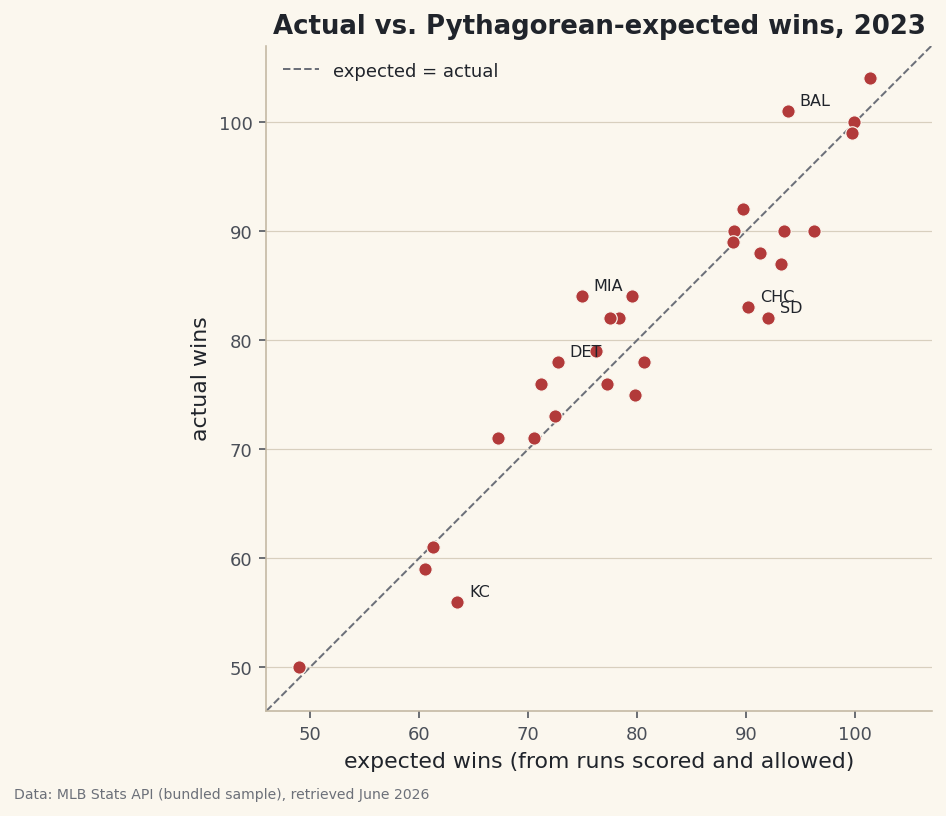
A scatter of actual vs. Pythagorean-expected wins that flags 2023's luckiest and unluckiest teams.
A team's win–loss record is the number everyone quotes, and it is one of the noisiest summaries in sports. Win a fistful of one-run games and your record races ahead of how you actually played; lose those coin-flips and it hides a good team. Pythagorean expectation cuts through the noise by asking a different question: given how many runs a team scored and allowed, how many games should it have won? Compute that for all 30 teams from the bundled 2023 standings, plot expected wins against real ones, and the luckiest and unluckiest teams in baseball fall straight out of the scatter.
This builds on Pandas for Sports Data: you should be comfortable loading a CSV and making a new column. The data is the same real sample_standings.csv (2023 MLB regular season, MLB Stats API, retrieved June 2026), so this runs offline.
-
Load the standings
The bundled file already has everything we need: games played (
G), wins (W), runs scored (RS), and runs allowed (RA).python import pandas as pd df = pd.read_csv("sample_standings.csv") print(df[["Team", "G", "W", "RS", "RA"]].head().to_string())Run differential — runs scored minus runs allowed — is the raw material here. The whole idea of Pythagorean expectation is that the ratio of runs scored to runs allowed maps cleanly onto winning percentage.
-
The Pythagorean formula
Bill James named it after the Pythagorean theorem because his first version squared each term. The expected winning percentage is:
python EXP = 1.83 # the refined exponent that best fits modern baseball df["ExpWinPct"] = df["RS"]**EXP / (df["RS"]**EXP + df["RA"]**EXP)The original exponent was a clean
2; analysts later found that 1.83 fits real baseball outcomes a little better, so that's what we use. The structure is intuitive: if a team scores exactly as many runs as it allows, the formula returns .500. The moreRSoutweighsRA, the closer the expected percentage climbs toward 1.000. -
Turn it into expected wins, and measure luck
Multiply the expected winning percentage by games played to get expected wins, then subtract from real wins. That gap — we'll call it
Luck— is how many games a team won beyond what its run differential earned.python df["ExpW"] = (df["ExpWinPct"] * df["G"]).round(1) df["Luck"] = (df["W"] - df["ExpW"]).round(1) # +ve = won more than expected ranked = df.sort_values("Luck", ascending=False) print(ranked[["Team", "W", "ExpW", "Luck", "RS", "RA"]].head().to_string())Luckiest and unluckiest teams, 2023Luckiest teams in 2023 (most wins above Pythagorean expectation): Team W ExpW Luck RS RA 11 Marlins 84 74.9 9.1 666 723 1 Orioles 101 93.8 7.2 807 678 18 Tigers 78 72.7 5.3 661 740 21 Pirates 76 71.2 4.8 692 790 12 D-backs 84 79.5 4.5 746 761 Unluckiest teams (most wins below expectation): Team W ExpW Luck RS RA 14 Padres 82 92.0 -10.0 752 648 28 Royals 56 63.5 -7.5 676 859 13 Cubs 83 90.2 -7.2 819 723 10 Twins 87 93.2 -6.2 778 659 7 Rangers 90 96.2 -6.2 881 716The 2023 Marlins are the poster child: they were outscored on the season (666 runs for, 723 against) yet went 84–78, winning about nine more games than their run differential expected. At the other extreme, the Padres scored 752 and allowed just 648 — the profile of a ~92-win team — but finished 82–80, ten wins short. A useful reminder that Pythagorean luck is about the regular season: the Rangers also underperformed their expectation here, then got hot in October and won the World Series.
-
Plot expected vs. actual wins
A scatter with a 45-degree reference line makes luck visible at a glance: teams above the line won more than expected, teams below it less.
python import matplotlib.pyplot as plt fig, ax = plt.subplots(figsize=(8, 6)) ax.scatter(df["ExpW"], df["W"], color="#B23A3A", s=45, zorder=3) lo, hi = 45, 110 ax.plot([lo, hi], [lo, hi], color="#6C7079", ls="--", label="expected = actual") ax.set_aspect("equal") ax.set_xlabel("expected wins (from runs scored and allowed)") ax.set_ylabel("actual wins") fig.savefig("expected_vs_actual.png", dpi=144, bbox_inches="tight")Data: Bundled sample (2023 MLB standings), retrieved June 2026 Setting
ax.set_aspect("equal")matters here: because both axes are in the same unit (wins), an equal aspect ratio keeps the 45-degree line at a true 45 degrees, so "distance from the line" reads honestly as games of luck. Most teams hug the line — over a 162-game season, luck mostly washes out — which is exactly why the few that stray are worth a closer look.
Troubleshooting
My expected wins look slightly different from another site's
Almost certainly the exponent. The classic formula uses 2; we use 1.83; some sites use a "PythagenPat" exponent that varies with run environment. They all agree to within a game or two — the point is the gap between expected and actual, not the third decimal place.
The dashed line isn't at 45 degrees
The axes are on different scales or aspect ratios. Give both the same limits and call ax.set_aspect("equal") so one win is the same distance on each axis.
I get a division error or odd values
Make sure RS and RA are numeric (not text) — df.dtypes will tell you. A team with zero runs allowed would divide by a tiny number, but that never happens over a real season.
Challenge yourself
Recompute ExpW with the original exponent of 2 and add it as a second column next to the 1.83 version. How much do the two disagree — is it ever more than a game or two? Then sort by Luck and color the scatter points red for unlucky and green for lucky, so the story jumps out without reading any labels. For a stiffer test, apply the same idea to a sport with a different exponent: point differential predicts winning across most team sports, only the exponent changes.
Get the code
Here's the complete, working script for this tutorial. It runs exactly as shown.
Download the finished script (41_pythagorean_wins_expected_standings.py)This script imports a small shared helper (and reads any bundled sample data) that live next to it in /downloads/ — grab these into the same folder so it runs as-is: sdt_common.py.