Pull Your First MLB Data with pybaseball

The single best thing about baseball analytics is that the richest data in all of sports is free and sitting right there. Statcast - the camera-and-radar rig bolted into every MLB park, tracking the speed and spin and launch angle of literally every pitch and batted ball - is one Python import away. No API key, no scraping, no paywall. We'll install pybaseball, turn caching on so we're polite about it, pull a real week of pitches, and sit with the one fact that reframes how you think about this data: every row is one pitch. Then we'll chart how hard a week of big-league hitters actually struck the ball, just to prove the data is genuinely there.

This assumes you've already set up Python for sports analytics and worked through the twelve core pandas operations. If import pandas works on your machine, you're ready. The data here comes from Baseball Savant via pybaseball, retrieved June 2026.

1. Install pybaseball

   pybaseball is a community library that wraps Baseball Savant, FanGraphs, and Baseball-Reference behind tidy Python functions. Install it once from your terminal:

   pip install pybaseball

   That pulls in pandas and a few helpers if you don't already have them. Everything else in this tutorial happens inside a single Python script.

2. Turn on caching - be a good citizen

   Before we download anything, we enable pybaseball's on-disk cache. This is the most important habit in this whole series: a cache means that the second time you run your script, the data loads from your own hard drive instead of hitting Baseball Savant's servers again. You get a faster script and you stop hammering a free public resource that the whole community shares.

   import matplotlib.pyplot as plt
   import pybaseball as pyb
   
   # Be a good citizen: cache every pull to disk. Run once, and the data is reused after.
   pyb.cache.enable()

   You only ever need to call pyb.cache.enable() once, near the top of your script. From then on, identical requests are served from disk. Think of it as the courteous default for any data pull, not an optimization you bolt on later.

3. Pull a week of Statcast data

   The function statcast(start, end) downloads every tracked pitch between two dates. We'll grab the first week of June 2023. Behind the scenes, Statcast splits this into one request per day - so a week is seven requests the first time, and zero the next time thanks to our cache.

   # One week of the 2023 season. Statcast splits this into one request per day.
   data = pyb.statcast("2023-06-01", "2023-06-07")

   When you run this for the first time you'll see a small progress bar tick through the seven days. That's expected; give it twenty or thirty seconds. The result, data, is an ordinary pandas DataFrame - just a very wide one.

4. See how big - and how wide - the data is

   Let's look at the shape before anything else. The number of rows will surprise people who expect "a week of baseball" to be small.

   print("Rows (one per pitch):", f"{len(data):,}")
   print("Columns:", data.shape[1])

   Output

   Rows (one per pitch): 25,714
   Columns: 118

   Over twenty-five thousand rows for a single week, and more than a hundred columns per row. That's the headline lesson of this tutorial: each row is one pitch, not one game and not one player. A typical MLB game has around 300 pitches, and a week has dozens of games, so the rows add up fast. Every one of those 118 columns describes some measured property of that single pitch - its speed, its spin, where it crossed the plate, and, if it was hit, how hard and at what angle it left the bat.

5. Look at a handful of real pitches

   A hundred-plus columns is too many to read at once, so we'll pick six that tell a clear story and print a few rows. We also drop pitches that were never put in play, because we want to see batted-ball numbers here.

   cols = ["game_date", "player_name", "events", "launch_speed", "launch_angle", "pitch_type"]
   sdt.show_df(data[cols].dropna(subset=["launch_speed"]), n=6)

   Six real pitches that were put in play

          game_date     player_name     events  launch_speed  launch_angle pitch_type
   2038  2023-06-07  Chafin, Andrew  force_out         104.2           -19         FF
   2627  2023-06-07  Chafin, Andrew     single          83.9            21         SI
   2926  2023-06-07  Chafin, Andrew     single          98.8            11         FF
   3206  2023-06-07  Chafin, Andrew        NaN          47.2           -24         SL
   2229  2023-06-07   Weems, Jordan  field_out         102.5            38         SL
   2334  2023-06-07   Weems, Jordan        NaN          71.7            23         FF

   Read one row at a time. The first is a pitch from Andrew Chafin - a four-seam fastball (FF) that was hit at 104.2 mph and turned into a force out. The player_name column here is the pitcher, a quirk of Statcast worth remembering. The events column is empty (NaN) on pitches that didn't end a plate appearance, which is why some batted balls show no event. And launch_speed - exit velocity in miles per hour - is the column we'll build the rest of this tutorial on.

6. Keep only the batted balls

   To talk about exit velocity, we need pitches that were actually struck. A pitch that was taken for a ball has no exit velocity, so its launch_speed is NaN. Dropping those rows leaves us with the batted balls, and a quick summary tells us we're in sane territory.

   # "launch_speed" is exit velocity in mph. Keep the rows that are actually batted balls.
   batted = data.dropna(subset=["launch_speed"])
   print("Batted balls this week :", f"{len(batted):,}")
   print("Average exit velocity  :", round(batted["launch_speed"].mean(), 1), "mph")
   print("Hardest-hit ball       :", round(batted["launch_speed"].max(), 1), "mph")

   Output

   Batted balls this week : 8,324
   Average exit velocity  : 83.0 mph
   Hardest-hit ball       : 116.6 mph

   Eight thousand batted balls in a week, averaging 83.0 mph off the bat, with the hardest one clocked at 116.6 mph. That top number is the kind of rocket only a few hitters in the world can produce, and seeing it confirms the pipeline is pulling genuine Statcast measurements - not something we could have invented.

7. Chart the distribution of exit velocity

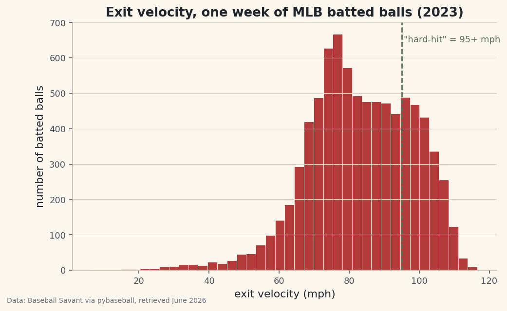
   A single average hides the shape of the data. A histogram shows it: we bucket every batted ball by how hard it was hit and count how many landed in each bucket. We'll also draw a dashed line at 95 mph, the conventional threshold for a "hard-hit" ball.

   fig, ax = plt.subplots(figsize=(7.8, 4.6))
   ax.hist(batted["launch_speed"], bins=40, color=sdt.sport_color("baseball"),
           edgecolor="#FBF7EE", linewidth=0.4)
   ax.axvline(95, color=sdt.SPORT_COLORS["foundations"], linestyle="--", linewidth=1.4)
   ax.text(95.6, ax.get_ylim()[1] * 0.92, '"hard-hit" = 95+ mph', fontsize=9,
           color=sdt.SPORT_COLORS["foundations"])
   ax.set_title("Exit velocity, one week of MLB batted balls (2023)")
   ax.set_xlabel("exit velocity (mph)")
   ax.set_ylabel("number of batted balls")
   fig.savefig("exit_velo_hist.png", dpi=144, bbox_inches="tight")

   

   Notice the shape: it isn't a tidy bell curve. There's a long tail of soft contact on the left - mishit grounders and broken-bat bloopers - and a denser cluster of hard contact bunched up near the right edge, because there's a physical ceiling on how hard a human can hit a baseball. The 95 mph line shows you, at a glance, what fraction of contact counts as "hard-hit." That single picture is the foundation for a lot of hitting analysis.

Troubleshooting