Monte Carlo: How Much Does Luck Move a Season's Record?

Here's a fact that should bother you a little: two teams with the exact same true talent can finish a season ten games apart in the standings, and neither did anything differently. That gap is luck. The way you measure it is Monte Carlo simulation — run the same random process thousands of times and look at the range of what comes out. It's the engine inside every playoff-odds model, and once you've built one, regression to the mean stops being a slogan and becomes arithmetic.

This builds on Summary Statistics and Distributions. The data is the bundled sample_standings.csv (real 2023 MLB standings), so it runs offline.

1. One season is a string of coin flips

   Treat a team's winning percentage as its "true talent" — the probability it wins any given game. A 162-game season is then 162 weighted coin flips, and the win total is a draw from a binomial distribution. A fixed seed makes the whole thing reproducible.

   import numpy as np
   import pandas as pd
   
   df = pd.read_csv("sample_standings.csv")
   rng = np.random.default_rng(2026)      # fixed seed -> same result every run
   
   best = df.loc[df["WinPct"].idxmax()]                       # the best team
   avg  = df.loc[(df["WinPct"] - 0.5).abs().idxmin()]         # a ~.500 team
   
   def simulate(p, games=162, trials=20000):
       return rng.binomial(games, p, size=trials)             # one number = one season's wins

   That's the whole model: rng.binomial(162, p, 20000) plays twenty thousand seasons for a team of talent p and hands back twenty thousand final win totals. No loop needed — numpy vectorizes it.

2. Read the spread, not the average

   The mean of the simulations just recovers the talent you put in (162 × p). The interesting part is the spread — the 5th-to-95th-percentile range tells you how far a record can drift on luck alone.

   for team, row in ((best["Team"], best), (avg["Team"], avg)):
       wins = simulate(row["WinPct"])
       lo, hi = np.percentile(wins, [5, 95])
       print(team, round(wins.mean(),1), "W,  90% range", int(lo), "-", int(hi))

   True talent in, a range of records out

   Braves     true talent 0.642  ->  mean 104.0 W, std  6.1, 90% range 94-114 (20 wins wide)
   Padres     true talent 0.506  ->  mean  82.0 W, std  6.4, 90% range 72-92 (20 wins wide)
   
   Same true talent, ~20-win spread: that gap is pure luck.

   Look at the width: even with talent held perfectly fixed, the 90% range is about 20 wins wide. A team can be a true 90-win club and finish anywhere from the low 80s to 100 without the underlying quality changing at all. That is why a hot or cold record over a partial season tells you much less than it feels like it should.

3. Picture the luck

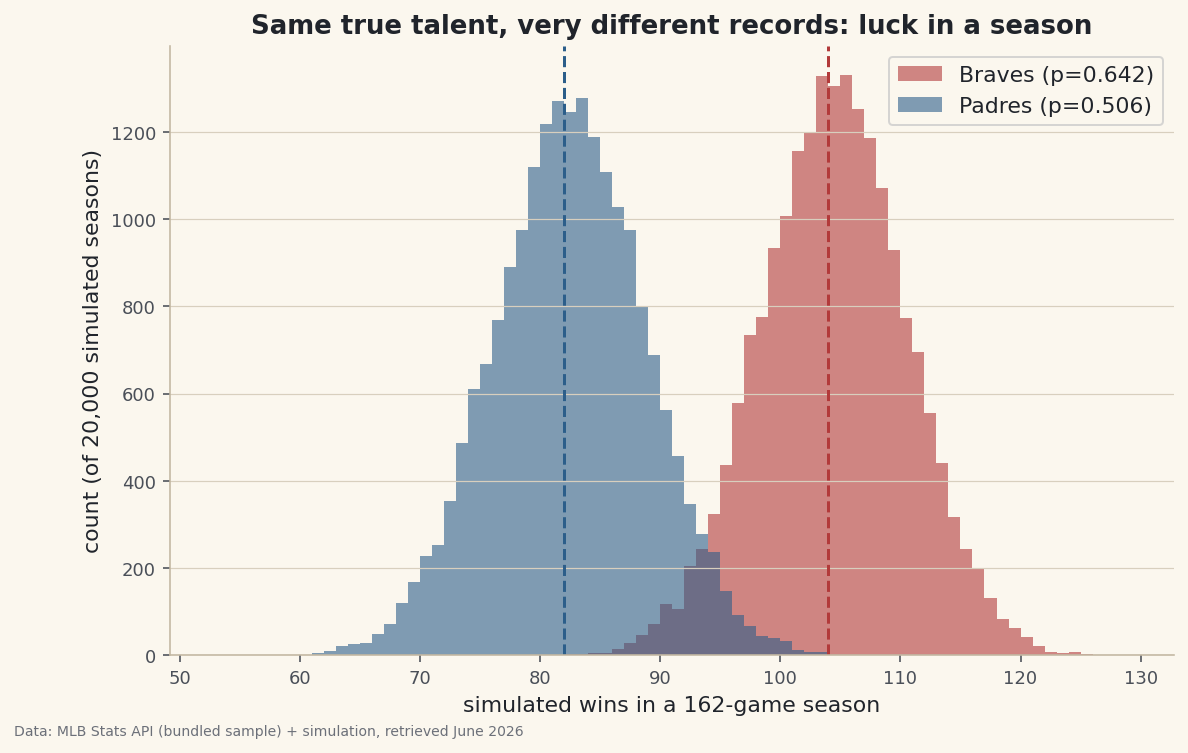
   Histogram the simulated win totals for both teams on the same axis and the overlap makes the point no table can: the tails of a good team and an average team reach into each other's territory.

   import matplotlib.pyplot as plt
   
   fig, ax = plt.subplots(figsize=(9, 5.5))
   for team, row, color in ((best["Team"], best, "#B23A3A"), (avg["Team"], avg, "#2C5E8A")):
       wins = simulate(row["WinPct"])
       ax.hist(wins, bins=range(60, 120), alpha=0.6, color=color, label=team)
       ax.axvline(wins.mean(), color=color, ls="--")
   ax.set_xlabel("simulated wins"); ax.legend()
   fig.savefig("season_spread.png", dpi=144, bbox_inches="tight")

   

   This same loop scales to anything you can assign a probability: simulate a full league of teams and count how often each makes the playoffs, and you've built a playoff-odds model. The honest version always reports the distribution, never a single confident number — because, as the chart shows, the single number was never the whole story.

Troubleshooting