Train/Test Split and the Confusion Matrix: Grading a Classifier Honestly

In the logistic-regression tutorial we trained a classifier to predict the NBA home win and reported that it was right 67% of the time. But we graded it on the same games it learned from — an open-book exam where the model had already seen every answer. The honest question is how it does on games it has never seen. That's what a train/test split answers, and the confusion matrix tells you what kind of mistakes it makes when a single accuracy number won't.

We reuse tutorial 71's setup exactly — predict the home win from the net-rating gap — on the bundled nba_ratings.csv and nba_home_results.csv, in pure numpy, offline.

Go deeper with the free textbook: Chapter 29: Evaluating Models — Accuracy, Precision, Recall at DataField.dev.

1. Hold out a test set the model never sees

   Shuffle the games with a fixed seed (so the tutorial is reproducible) and slice off 75% to train on and 25% to test on. The model will learn from the training games only; the test games are locked in a drawer until grading time.

   import numpy as np, pandas as pd
   # ... build x_all (net-rating gap, standardized) and y_all (home win) as in tutorial 71 ...
   
   rng = np.random.default_rng(72)
   idx = rng.permutation(len(x_all))
   cut = int(0.75 * len(x_all))
   tr, te = idx[:cut], idx[cut:]          # train indices, test indices
   x_tr, y_tr = x_all[tr], y_all[tr]
   x_te, y_te = x_all[te], y_all[te]

   The split

   Total games: 1231
   Train: 923   Test (held out): 308
   Home-win rate -> train 54.9% | test 52.6%

   Roughly 920 games to learn from, 300 held out. The home-win rate is about the same in both halves — a quick sanity check that the random split didn't accidentally hand us a lopsided test set.

2. Train on the training set only

   Exactly the gradient descent from tutorial 71 — but it only ever touches x_tr and y_tr. The test games are invisible to it.

   def sigmoid(z): return 1.0 / (1.0 + np.exp(-z))
   
   w, b, lr = 0.0, 0.0, 0.3
   for _ in range(400):
       p = sigmoid(w * x_tr + b)
       err = p - y_tr
       w -= lr * np.mean(err * x_tr)
       b -= lr * np.mean(err)

   That's the whole training step. Now — and only now — do we open the drawer.

3. Grade it honestly

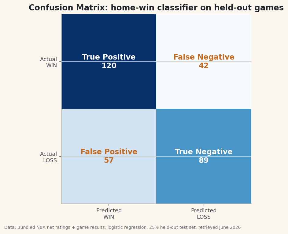
   Score the model on both halves. The number that matters is the test accuracy: performance on games it never trained on.

   acc_tr = ((sigmoid(w*x_tr + b) >= 0.5) == y_tr).mean()
   acc_te = ((sigmoid(w*x_te + b) >= 0.5) == y_te).mean()

   Honest evaluation

   Accuracy on TRAIN games: 67.5%
   Accuracy on TEST games:  67.9%   <- the honest number
   
   Confusion matrix (test set, positive = home win):
                    pred WIN   pred LOSS
     actual WIN        120          42
     actual LOSS        57          89
   
   Precision (of predicted wins, how many were right): 67.8%
   Recall (of real wins, how many we caught):          74.1%
   F1 score: 0.708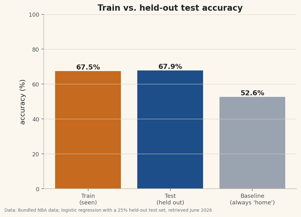

   

   Train and test accuracy are almost identical (about 67.5% vs 67.9%). That's the signature of a model that generalizes: it learned a real pattern, not the noise of specific games. A model that scored 90% on training and 60% on test would be overfitting — memorizing instead of learning. Our two-parameter model is too simple to overfit, which is a feature here. Both clear the “always pick home” baseline of about 53%.

4. Past accuracy: the confusion matrix

   Accuracy hides what kind of mistakes a model makes. The confusion matrix splits every test prediction into four boxes — correct wins (true positives), correct losses (true negatives), and the two ways to be wrong.

   pred = (sigmoid(w*x_te + b) >= 0.5).astype(int)
   tp = int(np.sum((pred==1) & (y_te==1)))   # said WIN, was WIN
   fp = int(np.sum((pred==1) & (y_te==0)))   # said WIN, was LOSS
   fn = int(np.sum((pred==0) & (y_te==1)))   # said LOSS, was WIN
   tn = int(np.sum((pred==0) & (y_te==0)))   # said LOSS, was LOSS

   

   Read the diagonal (120 + 89 correct) against the off-diagonal (57 + 42 wrong). Notice the model leans toward predicting “home win” — it has more false positives (57) than false negatives (42), because home teams win more often, so guessing “home” is the safer bet.

5. Precision, recall, and F1

   The four boxes give you the metrics accuracy can't. Precision: when the model says “home win,” how often is it right? Recall: of all the actual home wins, how many did it catch? F1 blends the two.

   precision = tp / (tp + fp)     # of predicted wins, share correct
   recall    = tp / (tp + fn)     # of real wins, share caught
   f1 = 2*precision*recall / (precision + recall)

   Here precision is about 68% and recall about 74% — the model catches three-quarters of real home wins but pays for it with some false alarms. That precision/recall trade is invisible in the single accuracy number, and it's exactly what you'd tune (by moving the 0.5 threshold) if false alarms cost more than misses, or vice versa.

Troubleshooting