Logistic Regression From Scratch: Predicting a Win, Not a Number

In the gradient-descent tutorial we taught a model to fit a straight line by stepping downhill on its error. A line is the right shape for predicting a number — wins, points, run differential. But plenty of the questions we actually care about are yes/no: did the home team win? A straight line answers that badly — it happily predicts a "probability" of 1.4 or −0.2, which is nonsense. Logistic regression fixes it with one small change: squash the line through a sigmoid so the output is always a real probability between 0 and 1, then learn the weights with the exact same downhill steps.

We'll build it from scratch in pure numpy to predict the NBA home win from a single feature — the gap in season net rating between the two teams. The data is bundled (nba_ratings.csv and nba_home_results.csv, 1,231 real games), so it runs offline.

Go deeper with the free textbook: Chapter 27: Logistic Regression and Classification at DataField.dev.

1. Build the dataset: a gap, and a yes/no

   The feature is how much better the home team is by season net rating; the label is whether it won. We standardize the feature to a z-score so a single learning rate behaves — the same habit from gradient descent.

   import numpy as np, pandas as pd
   
   ratings = pd.read_csv("nba_ratings.csv")
   nrtg = dict(zip(ratings.Team, ratings.NRtg))
   g = pd.read_csv("nba_home_results.csv")
   g["gap"] = g.home_team.map(nrtg) - g.away_team.map(nrtg)   # home edge
   g["home_win"] = (g.home_pts > g.away_pts).astype(int)       # the target
   
   x = ((g.gap - g.gap.mean()) / g.gap.std()).to_numpy()
   y = g.home_win.to_numpy().astype(float)

   What we're predicting

   Games: 1231
   Home teams won 54.3% of them (the baseline to beat).
   Net-rating gap ranges from -22.3 to 22.3 points.

   Home teams win 54.3% of the time — that's the baseline any model has to beat. Always guessing "home wins" is right 54.3% of the time; if our model can't do better, it's learned nothing.

2. The sigmoid: a line that can't escape 0 and 1

   The whole trick is one function. Take the linear score z = w·x + b — which can be any number from −∞ to +∞ — and pass it through the sigmoid. Big positive z → near 1; big negative → near 0; z = 0 → exactly 0.5. Now the output is always a valid probability.

   def sigmoid(z):
       return 1.0 / (1.0 + np.exp(-z))

   That S-shape is the entire difference between linear and logistic regression. Everything else — the gradient descent, the loss curve — is the same machinery you already built.

3. The right loss for a probability: log-loss

   Mean squared error is the wrong tool here; for classification we use log-loss (cross-entropy), which punishes confident wrong answers hard and rewards confident right ones. The beautiful part: when you predict with a sigmoid and score with log-loss, the gradient simplifies to exactly the same form as before — (prediction − truth) times the input.

   w, b = 0.0, 0.0
   lr = 0.3
   losses = []
   for step in range(400):
       p = sigmoid(w * x + b)                       # predicted probabilities
       losses.append(-np.mean(y*np.log(p+1e-12) + (1-y)*np.log(1-p+1e-12)))
       err = p - y                                  # same gradient shape as linear!
       w -= lr * np.mean(err * x)
       b -= lr * np.mean(err)

   Predict, measure the error, step downhill, repeat — the identical skeleton from gradient descent. Only the prediction function (sigmoid) and the loss (log-loss) changed.

4. Watch the log-loss fall

   Same diagnostic as always: plot the loss against the training step. A healthy run drops fast then flattens.

   import matplotlib.pyplot as plt
   fig, ax = plt.subplots()
   ax.plot(losses)
   ax.set_xlabel("step"); ax.set_ylabel("log-loss")
   fig.savefig("logit_loss.png", dpi=144, bbox_inches="tight")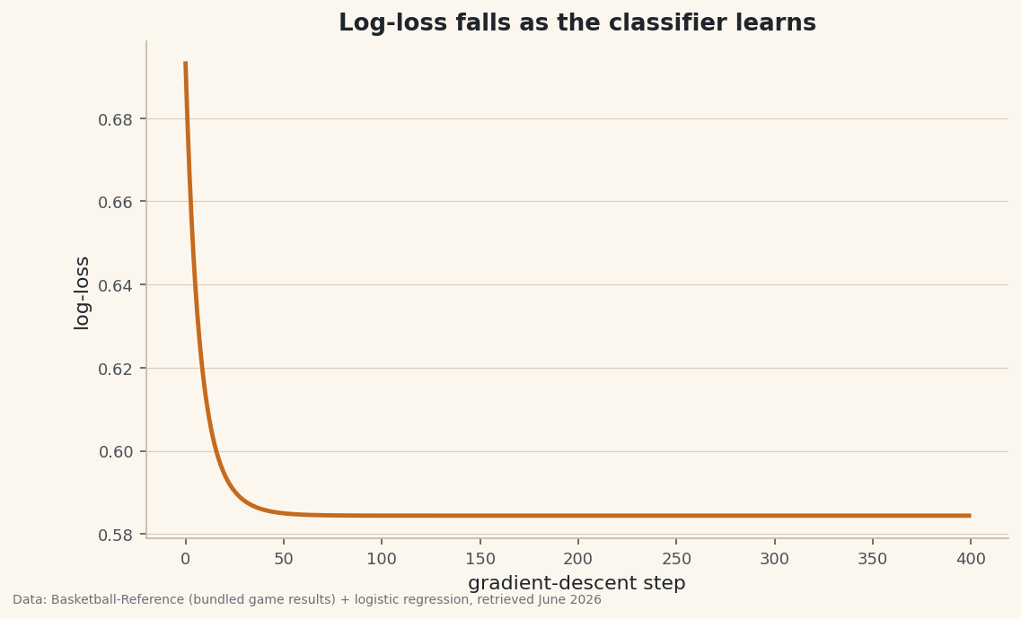

   

   It starts at 0.693 — that's the log-loss of a coin flip, the model knowing nothing — and settles near 0.584. The drop is the model learning that a bigger net-rating gap means a more likely home win.

5. See the S-curve trace the real win rates

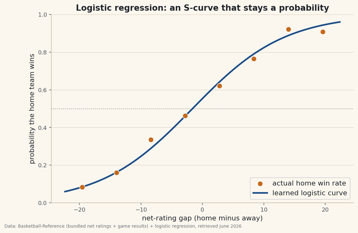
   Now plot the learned curve over the data. Bucket the games by net-rating gap and mark each bucket's actual home win rate; the logistic curve should thread right through them.

   fig, ax = plt.subplots()
   gx = np.linspace(g.gap.min(), g.gap.max(), 200)
   gz = (gx - g.gap.mean()) / g.gap.std()
   ax.plot(gx, sigmoid(w * gz + b))     # the learned probability curve
   ax.set_ylim(0, 1)
   fig.savefig("logit_curve.png", dpi=144, bbox_inches="tight")

   

   The dots are reality; the curve is the model. When the home team is much worse (a gap of −20) it wins only about a fifth of the time; when it's much better (+20) it wins over 80%. At a gap of zero the curve sits just above 0.5 — the residual home-court edge after talent is equal.

6. How good is it? Beat the baseline

   Turn probabilities into yes/no by thresholding at 0.5, then check accuracy against the truth.

   acc = ((sigmoid(w*x + b) >= 0.5) == y).mean()

   The trained classifier

   Start log-loss:      0.6931
   After 400 steps:     0.5844
   Learned weight w = 1.064, intercept b = 0.217
   Accuracy: 67.3% (vs 54.3% from always guessing 'home wins')
   A home team +6 in net rating is predicted to win 73% of the time.

   The model is right 67.3% of the time — a real 13-point lift over the 54.3% you'd get from always guessing "home wins." And it's interpretable: a home team six net-rating points better than its opponent is predicted to win about 73% of the time. One feature, one S-curve, and you've got a calibrated win-probability model.

Troubleshooting