Gradient Descent From Scratch: How Models Actually Learn

Back in the regression tutorial we fit a line with a one-shot formula. That's a luxury — most machine-learning models have no closed-form answer and have to learn it instead, by starting with a bad guess and nudging it downhill until the error stops shrinking. That process is gradient descent, and it's the engine under almost every model you'll meet. We'll build it from scratch in pure numpy, watch the loss fall step by step, and confirm it arrives at the exact same line the formula gives.

This builds on Z-Scores (we standardize so one learning rate works) and pairs with k-means (another algorithm that loops to a solution). The data is the bundled sample_standings.csv (real 2023 MLB standings), so it runs offline.

Go deeper with the free textbook: Linear Regression: Your First Predictive Model at DataField.dev.

1. Set up the problem

   We'll learn the line from run differential to wins. Standardize both to z-scores first — that puts them on a common scale so a single learning rate behaves, and it's a habit worth keeping for gradient descent.

   import numpy as np, pandas as pd
   
   df = pd.read_csv("sample_standings.csv")
   x = ((df.RunDiff - df.RunDiff.mean()) / df.RunDiff.std()).to_numpy()
   y = ((df.W - df.W.mean()) / df.W.std()).to_numpy()
   m, b = 0.0, 0.0          # start with a flat line: slope 0, intercept 0

   The descent, start to finish

   Start loss: 0.9667
   After 200 steps: 0.1056
   Learned slope m = 0.944, intercept b = -0.000
   Closed-form (numpy.polyfit): slope 0.944, intercept 0.000
   Gradient descent landed on the same line - it just walked there.

2. The idea: roll downhill on the error surface

   Pick a loss — mean squared error, the average squared gap between prediction and truth. For any line (m, b) the loss is some height on a bowl-shaped surface. Gradient descent computes the slope of that bowl (the gradient) and steps in the downhill direction. Do it enough times and you reach the bottom: the best-fit line.

   lr = 0.1                       # learning rate: how big each step is
   losses = []
   for step in range(200):
       pred = m * x + b
       err = pred - y
       losses.append(np.mean(err ** 2))     # current loss
       dm = 2 * np.mean(err * x)            # gradient w.r.t. slope
       db = 2 * np.mean(err)               # gradient w.r.t. intercept
       m -= lr * dm                         # step downhill
       b -= lr * db

   That's the whole algorithm: predict, measure the error, compute the two gradients, take a small step against them, repeat. No formula for the answer — just thousands of tiny corrections.

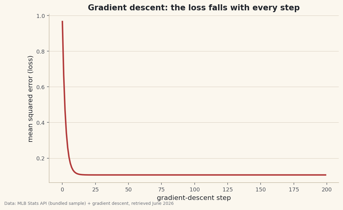
3. Watch the loss fall

   The single most useful plot in machine learning is the loss curve: error against training step. A healthy run drops fast, then flattens as it nears the bottom.

   import matplotlib.pyplot as plt
   fig, ax = plt.subplots()
   ax.plot(losses)
   ax.set_xlabel("step"); ax.set_ylabel("mean squared error")
   fig.savefig("gd_loss.png", dpi=144, bbox_inches="tight")

   

   Ours drops from 0.97 to 0.11 and levels off — the line has stopped improving. That flattening is how you know to stop training.

4. Confirm it learned the right line

   Gradient descent isn't magic — for a straight line it should land exactly where the closed-form formula does. It does: a learned slope of 0.944, matching numpy.polyfit to three decimals. It just walked there instead of solving it in one step.

   fig, ax = plt.subplots()
   ax.scatter(x, y)
   xs = np.linspace(x.min(), x.max(), 50)
   ax.plot(xs, m * xs + b)        # the learned line
   fig.savefig("gd_fit.png", dpi=144, bbox_inches="tight")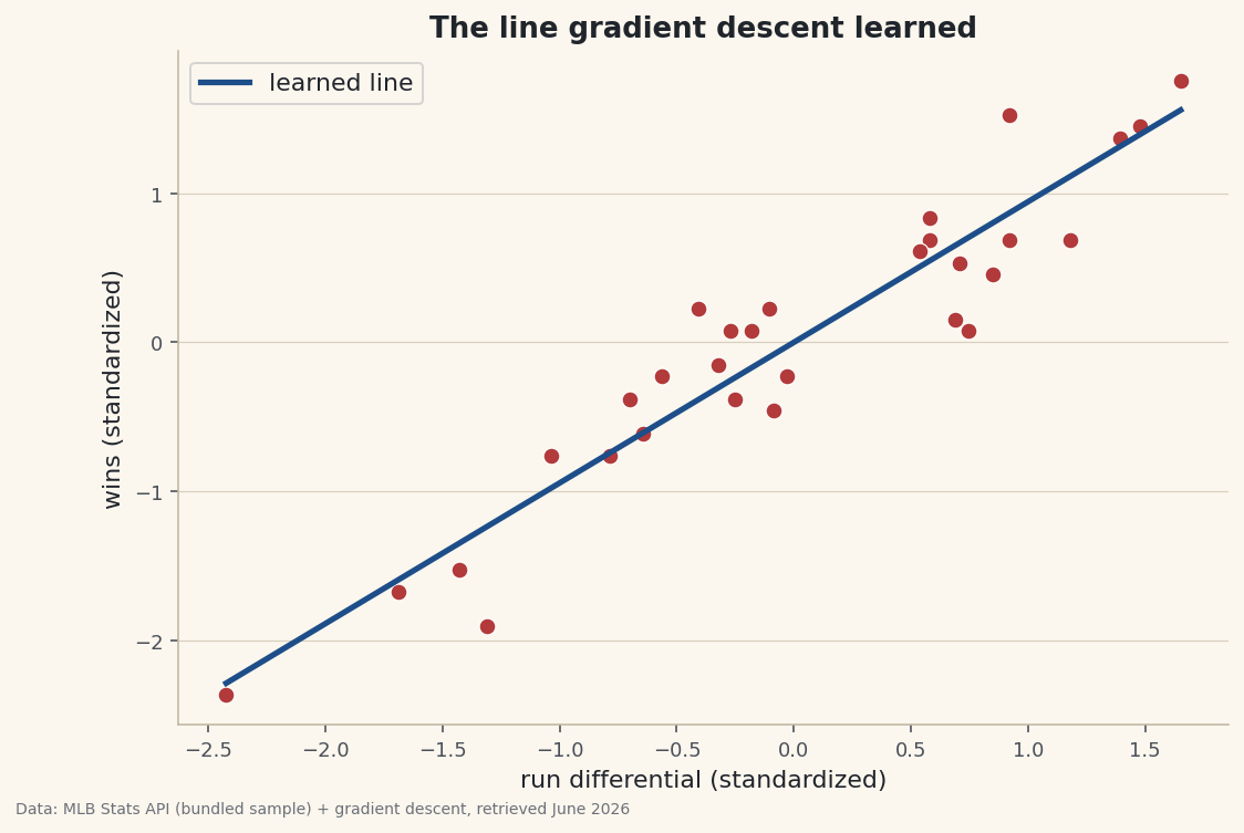

   

   The payoff: this same loop fits models that have no formula — logistic regression, neural networks, everything. Swap the prediction and the loss; the predict-measure-step-repeat skeleton never changes.

Troubleshooting