A Decision Tree From Scratch

The logistic regression and the k-nearest neighbors models both predicted the NBA home win well, but neither is something you can explain to a friend. A decision tree is: it's a flowchart of yes/no questions on the features, and you can read every branch. We grow one from scratch in pure numpy — choosing each split to make the two sides as “pure” as possible — on the same two features (home net rating, away net rating), then compare it to the earlier models and read the tree it learned.

Go deeper with the free textbook: Chapter 28: Decision Trees and Random Forests at DataField.dev.

1. Measure purity with Gini impurity

   A split is good if each side ends up mostly one class. Gini impurity measures how mixed a group of labels is: 0 means perfectly pure (all home wins or all losses), 0.5 means a 50/50 coin-flip mix. The whole tree is built by finding splits that lower it.

   import numpy as np
   
   def gini(y):
       if len(y) == 0:
           return 0.0
       p = y.mean()                 # share of home wins
       return 1.0 - (p**2 + (1 - p)**2)

   A group that's 90% home wins has a Gini of 0.18; a 50/50 group has 0.50. Lower is purer.

2. Find the best split by brute force

   For every feature and every candidate threshold, we split the data in two and measure the weighted Gini of the children. The split that lowers impurity the most wins. With two features and a few hundred games, brute force is plenty fast.

   def best_split(X, y):
       best = (None, None, gini(y))                 # (feature, threshold, impurity)
       for f in range(X.shape[1]):
           for thr in np.unique(X[:, f]):
               left = X[:, f] <= thr
               if left.sum() == 0 or (~left).sum() == 0:
                   continue
               imp = left.mean()*gini(y[left]) + (~left).mean()*gini(y[~left])
               if imp < best[2]:
                   best = (f, thr, imp)
       return best

   That's the engine. The feature and threshold it returns is the single question that best separates home wins from losses at this node.

3. Recurse to grow the tree

   A tree is just that split, applied again to each side, until a stopping rule: a maximum depth, or too few games left to split. Each leaf predicts the majority class of the games that reach it. We cap depth at 3 so the tree stays readable and doesn't overfit.

   def grow(X, y, depth, max_depth=3, min_leaf=20):
       node = {"pred": int(round(y.mean())), "p": float(y.mean()), "n": len(y)}
       if depth >= max_depth or len(y) < 2*min_leaf or gini(y) == 0:
           return node                              # make a leaf
       f, thr, _ = best_split(X, y)
       left = X[:, f] <= thr
       if left.sum() < min_leaf or (~left).sum() < min_leaf:
           return node
       node["feat"], node["thr"] = f, thr
       node["left"]  = grow(X[left],  y[left],  depth+1, max_depth, min_leaf)
       node["right"] = grow(X[~left], y[~left], depth+1, max_depth, min_leaf)
       return node

   To predict, you walk from the root: at each node, go left if the feature is at or below the threshold, right otherwise, until you hit a leaf and read its prediction.

4. Read the tree and score it

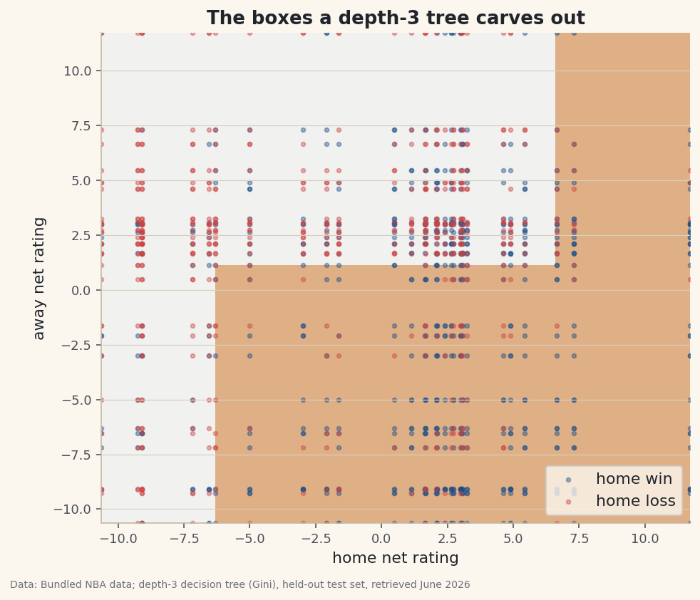
   the learned decision tree

   Decision tree (max depth 3), trained on 923 games:
   
    if home net rating <= -6.3:
       then if away net rating <= -2.1:
           then leaf -> home loss (44% home win, n=71)
           else if away net rating <= 3.0:
               then leaf -> home loss (21% home win, n=89)
               else leaf -> home loss (8% home win, n=63)
       else if away net rating <= 1.1:
           then if home net rating <= 4.6:
               then leaf -> HOME WIN (76% home win, n=238)
               else leaf -> HOME WIN (90% home win, n=73)
           else if home net rating <= 6.7:
               then leaf -> home loss (48% home win, n=357)
               else leaf -> HOME WIN (84% home win, n=32)
   
   Held-out test accuracy: 64.6%  (guess-home baseline 55.2%)
   Compare: logistic regression ~64%%, k-NN ~66%% on the same problem.
   The tree is less accurate but fully readable - you can follow every decision.

   

   The tree scores 64.6% on the held-out test set — right alongside the logistic regression (~64%) and just behind k-NN (~66%), and well above the 55% you'd get by always guessing the home team. But the real payoff is in the printout: you can follow every decision. If the home team's net rating is deeply negative, it predicts a loss; if the home team is strong and the away team is weak, it predicts a win, with a confidence (the leaf's home-win rate) attached. The chart shows the same thing geometrically — the tree carves the feature space into rectangular boxes and votes within each.

5. The trade-off: readable vs. accurate

   A single shallow tree is the most interpretable model in this series and one of the least accurate — those hard rectangular splits can't capture a smooth, diagonal boundary the way logistic regression's line does. That's the classic tension. The fix in practice is to grow many trees on slightly different samples and average them — a random forest — which keeps most of the accuracy while giving up some of the readability. Build the one tree first; the forest is just a crowd of them.

Troubleshooting