Fourth-Down Decisions: Which Teams Go For It?

Which coaches actually trust the math on fourth down? For most of football history the choice was simple - punt, kick the field goal, or, only in desperation, go for it. Then the win-probability models started saying coaches were leaving points on the field, and a quiet arms race began. Here I put a number on it: filter a full 2023 season of play-by-play down to the fourth downs that reveal a coach's true philosophy, classify each decision as go / punt / kick, and rank every team by how often they went for it - the clearest single signal of analytics-era coaching.

This is an advanced tutorial, less because the code is hard and more because the filtering judgment is. It builds directly on EPA explained by building it - you'll want to be comfortable with the idea that a single number can value a decision before we start ranking decisions. As always we read nflverse's data through the sdt_nflverse helper rather than the broken nfl_data_py library. Data is nflverse play-by-play, retrieved June 2026.

1. Load four columns - including win probability

   We need only four facts per play: the offense, the down, what they did, and - the column that makes this analysis honest - the win probability at the moment of the snap. wp is nflverse's estimate, from 0 to 1, of the chance the team with the ball goes on to win the game.

   import matplotlib.pyplot as plt
   
   import sdt_common as sdt
   import sdt_nflverse as nfl
   
   sdt.init("fourth-down-decisions-who-goes-for-it")
   pbp = nfl.import_pbp_data([2023], columns=["posteam", "down", "play_type", "wp"])

   Win probability is the same family of model as EPA - it takes the full game state (score, time, field position, down) and outputs a single calibrated number. We'll use it not to value a play but as a filter, to throw out the situations where a coach's hand was forced and only intent, not philosophy, was on display.

2. Filter to fourth-down decisions

   First we keep only fourth downs, and only the four play types that represent a genuine decision: a pass or run (going for it), a punt, or a field-goal attempt. We drop everything else - penalties, aborted plays, kneels - because they aren't a clean choice.

   fourth = pbp[(pbp["down"] == 4)
                & (pbp["play_type"].isin(["pass", "run", "punt", "field_goal"]))].copy()

   The .copy() gives us a fresh DataFrame to add columns to without the SettingWithCopyWarning. At this point fourth holds every real fourth-down decision in the league, but it's not yet the fair set - that's the next, more important step.

3. Keep only competitive situations

   This is the judgment call that separates a thoughtful analysis from a misleading one. A team trailing by 20 in the fourth quarter goes for it on every fourth down out of desperation, not conviction; a team leading by 20 punts everything to run out the clock. Neither tells you what that coach believes. So we keep only plays where the win probability was between 5% and 95% - close enough that the decision reflects strategy rather than the scoreboard forcing his hand.

   # Keep competitive situations (win probability 5-95%) so we measure intent, not
   # end-of-game desperation or garbage time.
   fourth = fourth[fourth["wp"].between(0.05, 0.95)]
   fourth["go"] = fourth["play_type"].isin(["pass", "run"]).astype(int)

   The between(0.05, 0.95) call returns a boolean mask we use to slice - it's the readable way to express "inside this range." Then go becomes our 1/0 flag: 1 if the play was a pass or run (they went for it), 0 if it was a punt or field goal. As in the tendencies analysis, encoding a yes/no decision as 1/0 means the average of the column over any group is exactly the go-for-it rate for that group - a trick worth keeping in your back pocket.

4. Rank teams by go-for-it rate

   Now the ranking is a one-liner. We group by offense, take the mean of the go flag (the rate), scale to a percentage, round, and sort so the boldest teams sit at the bottom of the sorted Series - which is where matplotlib will want them for a horizontal bar chart.

   rate = (fourth.groupby("posteam")["go"].mean().mul(100).round(1).sort_values())

   Read this as a pipeline: groupby("posteam")["go"].mean() gives each team's go-for-it rate, .mul(100) turns it into a percentage, and .sort_values() orders it ascending. The whole chain fits on one line because each step hands a Series to the next - the fluent style you saw building leaderboards in the exit-velocity tutorial.

5. Read the extremes

   Let's print the boldest and most conservative teams, then the eight most aggressive offenses of the season.

   with sdt.snippet("rates"):
       print("Go-for-it rate on 4th down, competitive situations, 2023 (%):")
       print(f"Most aggressive: {rate.index[-1]} ({rate.iloc[-1]}%)   "
             f"Most conservative: {rate.index[0]} ({rate.iloc[0]}%)")
       print(rate.tail(8).to_string())

   Who actually goes for it

   Go-for-it rate on 4th down, competitive situations, 2023 (%):
   Most aggressive: DET (26.6%)   Most conservative: SF (5.7%)
   posteam
   WAS    20.0
   DAL    20.0
   ARI    20.6
   LAC    20.8
   PHI    21.4
   MIN    22.9
   CAR    24.4
   DET    26.6

   The spread here is the whole story. The Detroit Lions led the league, going for it 26.6% of the time in competitive situations - more than one fourth down in four. At the other end, the San Francisco 49ers went for it just 5.7% of the time, nearly a fivefold difference between the boldest and most cautious teams in the same league under the same math. That gap is not about which coach knows the numbers - by 2023 they all have the same models - it's about temperament and trust. Detroit's Dan Campbell turned fourth-down aggression into an identity. The .tail(8) shows the rest of the bold tier filling in behind Detroit: Carolina at 24.4%, Minnesota at 22.9%, Philadelphia at 21.4%, a cluster of teams that have bought in. These are real 2023 rates, retrieved June 2026. Note that 49ers at 5.7% being "conservative" partly reflects how often they led - even after filtering, a dominant team faces fewer toss-up fourth downs.

6. Chart the whole league

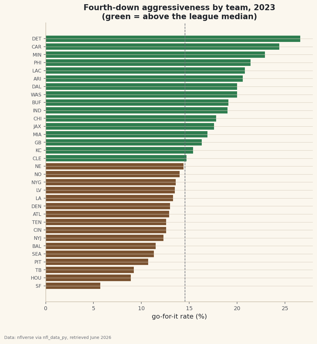
   A horizontal bar chart shows the full pecking order at once. We color teams above the league median in one color and below it in another, and draw a vertical line at the median so each team's position relative to the pack is instantly readable.

   fig, ax = plt.subplots(figsize=(8, 8.4))
   colors = [sdt.sport_color("football") if v < rate.median() else sdt.SPORT_COLORS["soccer"]
             for v in rate.values]
   ax.barh(rate.index, rate.values, color=colors)
   ax.axvline(rate.median(), color="#6C7079", linestyle="--", linewidth=1)
   ax.set_xlabel("go-for-it rate (%)")
   ax.set_title("Fourth-down aggressiveness by team, 2023\n(green = above the league median)")
   ax.tick_params(axis="y", labelsize=8)
   sdt.save_fig(fig, "fourth_down", source="nflverse via nfl_data_py")

   

   The color list is built with a comprehension that compares each team's rate to the median - green for the bold half, brown for the cautious half - so the chart sorts the league into two camps at a glance. The dashed median line is the visual spine: it's a more honest center than the mean here, because a couple of very aggressive teams would drag a mean upward and make the "average" team look bolder than it is. Reading the chart top to bottom, you can watch the analytics philosophy spread across the league as a gradient rather than a switch - there's no clean line where "old school" ends and "new school" begins, just a continuum of how much each staff trusts the fourth-down math.

Troubleshooting