Receiver Efficiency: Targets, Catches, and Yards After Catch

Look at any receiving leaderboard sorted by yards and you'll see the same thing: the players with the most yards are usually just the players who got thrown to the most. Volume and efficiency are different questions, and conflating them is how a busy possession receiver gets mistaken for a genuine difference-maker. So keep them on separate axes. We'll aggregate a full 2023 season of play-by-play down to the receiver level — targets, catch rate, yards, yards after the catch, and EPA per target — then draw a scatter with volume on one axis and efficiency on the other, so neither story can hide behind the other.

This is an intermediate step: we're moving from analyzing plays to analyzing people, which means collapsing many rows into one row per receiver. It builds on pulling your first NFL data, so I'll assume the sdt_nflverse helper is working and you know why we read nflverse's parquet directly instead of fighting the broken nfl_data_py library. The metric on the vertical axis, EPA, gets its own full treatment in EPA explained by building it if you want the deep version. Data is nflverse play-by-play, retrieved June 2026.

1. Load the target-level columns

   Every column we pull answers one question about a passing play: who was targeted, what team they're on, was it caught, how many yards it gained, how many of those came after the catch, the play's EPA, and a flag marking pass attempts. That last flag is what lets us isolate targets cleanly.

   import matplotlib.pyplot as plt
   
   import sdt_common as sdt
   import sdt_nflverse as nfl
   
   sdt.init("receiver-efficiency-targets-catches-yac")
   pbp = nfl.import_pbp_data([2023], columns=[
       "receiver_player_name", "posteam", "complete_pass", "yards_gained",
       "yards_after_catch", "epa", "pass_attempt"])

   A note on two of these columns. complete_pass is a 0/1 flag, so summing it counts catches. yards_after_catch (YAC) is the yardage a receiver earned with his legs after the ball arrived, separate from how far it traveled in the air - it's a real skill, and it's why a short-passing offense can still move the ball explosively.

2. Keep real targets only

   We want plays that were genuine pass attempts and had a named receiver. The receiver-name filter quietly drops throwaways, spikes, and scrambles where nobody was targeted, which would otherwise pollute the catch-rate math.

   targets = pbp[(pbp["pass_attempt"] == 1) & (pbp["receiver_player_name"].notna())]

   Notice we don't need a .copy() here because we never modify targets in place - we immediately feed it into a groupby on the next step, which produces a fresh DataFrame of its own. The receiver names arrive in an abbreviated form like T.Hill (first initial, last name), which is how nflverse stores them; it's compact and unambiguous enough for a leaderboard.

3. Aggregate to one row per receiver

   This is the central move. We group every target by the receiver, then compute six summaries at once with named aggregation - the team they play for, total targets, catches, total yards, total YAC, and their mean EPA per target. Then we require at least 70 targets so part-time players don't crowd the chart with noisy rate stats.

   rec = (targets.groupby("receiver_player_name")
          .agg(team=("posteam", "first"), targets=("pass_attempt", "sum"),
               catches=("complete_pass", "sum"), yards=("yards_gained", "sum"),
               yac=("yards_after_catch", "sum"), epa=("epa", "mean"))
          .query("targets >= 70"))

   The tuple syntax - targets=("pass_attempt", "sum") - reads as "make a column called targets by summing pass_attempt," and it lets us build all six columns in a single pass over the data. The mix of aggregations is deliberate: we sum the counting stats (targets, catches, yards), take the mean for the rate stat (EPA per target), and grab the team with first since it's the same on every row for a given player. The query("targets >= 70") is our sample-size floor - the same discipline as the minimum batted-balls rule in the Statcast exit-velocity leaderboard: a receiver with eight targets and four lucky catches has a meaningless 50% catch rate, and we don't want him near the top.

4. Derive the two efficiency rates

   The aggregated totals aren't comparable across players yet - of course a 200-target receiver has more catches than a 75-target one. We convert two of the totals into rates: catch percentage and yards-after-catch per reception.

   rec["catch%"] = (100 * rec["catches"] / rec["targets"]).round(1)
   rec["yac_per_rec"] = (rec["yac"] / rec["catches"]).round(1)

   Dividing one column by another is element-wise, so each receiver gets his own rate in one line. Catch percentage is catches over targets, a measure of reliability and the quality of throws he gets. YAC per reception divides total YAC by catches, not targets - because you can only gain yards after a catch on plays you actually caught - which makes it a clean per-reception skill number.

5. Read the efficiency leaderboard

   Let's sort by EPA per target - the purest single efficiency number here - and look at the ten most efficient high-volume receivers of the season.

   with sdt.snippet("leaders"):
       top = rec.sort_values("epa", ascending=False).head(10)
       print("Most efficient high-volume receivers, 2023 (min 70 targets):")
       print(top[["team", "targets", "catch%", "yards", "yac_per_rec", "epa"]].round(3).to_string())

   Efficiency, not just volume

   Most efficient high-volume receivers, 2023 (min 70 targets):
                        team  targets  catch%   yards  yac_per_rec    epa
   receiver_player_name                                                  
   B.Aiyuk                SF    125.0    67.2  1491.0          4.6  0.721
   G.Kittle               SF    103.0    70.9  1132.0          7.4  0.653
   N.Collins             HOU    127.0    71.7  1463.0          7.0  0.628
   D.Moore               CHI    149.0    69.8  1535.0          6.2  0.499
   T.Kelce                KC    158.0    79.1  1346.0          5.0  0.491
   C.Lamb                DAL    199.0    72.4  1861.0          5.0  0.488
   P.Nacua                LA    170.0    67.1  1667.0          6.5  0.485
   T.Hill                MIA    220.0    71.4  2152.0          5.2  0.452
   R.Doubs                GB    108.0    63.9   908.0          3.0  0.446
   A.Thielen             CAR    138.0    74.6  1016.0          3.3  0.440

   This list passes the smell test, which is how you know the pipeline is sound, and it rewards a close read. Brandon Aiyuk tops it at 0.721 EPA per target on 125 targets - elite value, and crucially not the highest-volume receiver in the league. Right behind him is his San Francisco teammate George Kittle, whose 7.4 YAC per reception is the highest in the top ten: a tight end turning short catches into long gains. Now find Tyreek Hill near the bottom of this list: he led everyone shown with 220 targets and 2,152 yards, yet his 0.452 EPA per target lands him below players who saw the ball far less. That's the entire lesson in one comparison - Hill's enormous yardage is partly a function of enormous volume, while Aiyuk produced more value on each individual target. Both are excellent; they're excellent in different ways, and a yards-only leaderboard would flatten that distinction. All of these are real 2023 season aggregates, retrieved June 2026.

6. Build the volume-versus-efficiency scatter

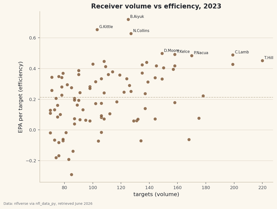
   Now the payoff chart, and the reason we kept volume and efficiency as separate numbers. Each receiver becomes a dot at his (targets, EPA) coordinates: the horizontal axis is how often he was thrown to, the vertical axis is how much value he produced per target. We add a dashed line at the league-average EPA so it's instantly clear who is above and below the bar, and we label the eight most efficient names.

   fig, ax = plt.subplots(figsize=(8.4, 6.2))
   ax.scatter(rec["targets"], rec["epa"], s=42, color=sdt.sport_color("football"),
              alpha=0.8, edgecolor="#FBF7EE", linewidth=0.4, zorder=3)
   ax.axhline(rec["epa"].mean(), color="#C2B7A1", linestyle="--", linewidth=1)
   for name, r in rec.sort_values("epa", ascending=False).head(8).iterrows():
       ax.annotate(name, (r["targets"], r["epa"]), fontsize=7.5,
                   xytext=(4, 3), textcoords="offset points")
   ax.set_xlabel("targets (volume)")
   ax.set_ylabel("EPA per target (efficiency)")
   ax.set_title("Receiver volume vs efficiency, 2023")
   sdt.save_fig(fig, "receiver_efficiency", source="nflverse via nfl_data_py")

   

   A few choices make this readable. The alpha=0.8 and pale edge let overlapping dots stay distinct in the crowded middle of the cloud. Labeling only the top eight - rather than every qualifying receiver - keeps the chart from turning into a wall of text; the names you most want to find are the ones near the top, and those are exactly the ones we annotate. The dashed mean line turns raw vertical position into meaning: everything above it is above-average efficiency. Read the chart by hunting for the upper area, and especially the upper-right: a dot that is both high and far to the right is the dream, a receiver staying efficient even while carrying a huge target load. A dot that is high but on the left is a hyper-efficient lower-volume option; a dot far right but low is a heavily-targeted player whose per-target value is ordinary. None of that geometry is visible in a yards column.

Troubleshooting