Measuring Inequality: Lorenz Curves and the Gini Coefficient
What you'll build
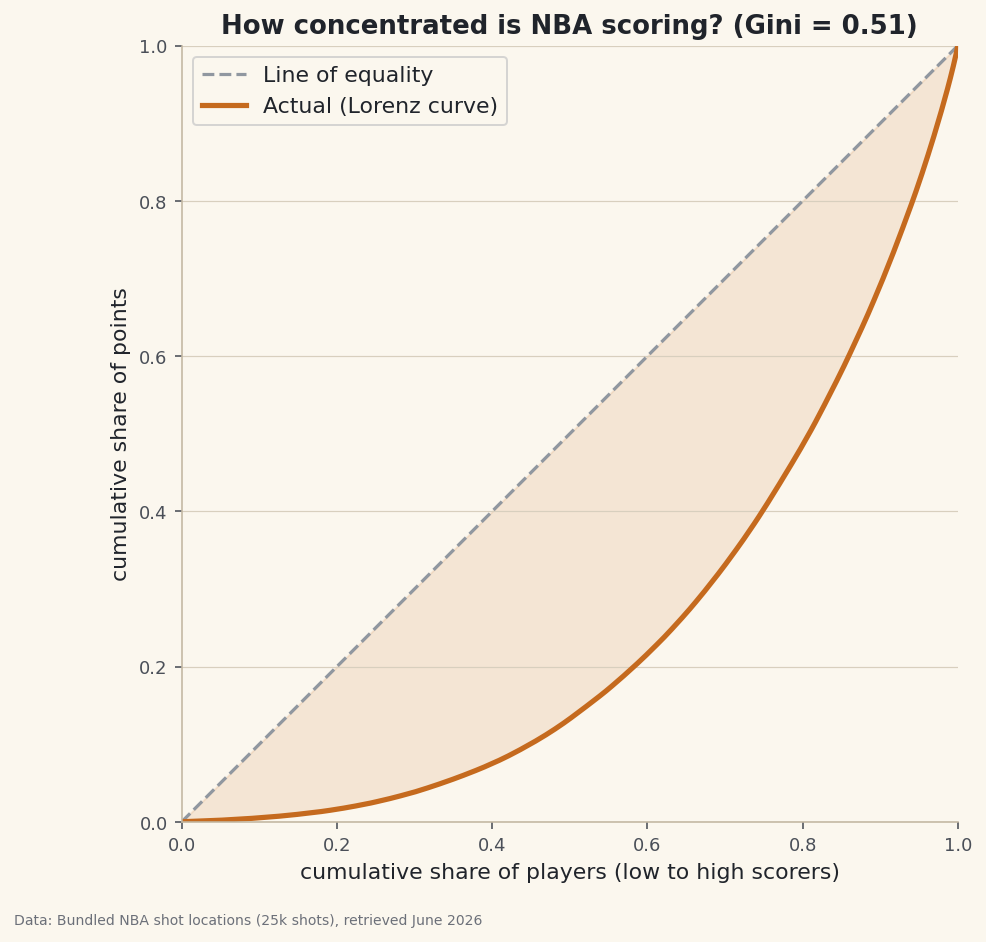
A Lorenz curve and Gini coefficient of NBA scoring, showing what share of points the top scorers actually account for.
"A handful of stars score most of the points." Everyone says it; almost nobody measures it. The tools that do are borrowed from economics, where they measure income inequality: the Lorenz curve and the Gini coefficient. They turn a vague sense of "concentration" into a picture and a single number — and they're pure numpy, just sorting and a cumulative sum. Once you have them, you can measure concentration in anything: scoring, salaries, shot attempts, minutes.
This builds on Summary Statistics and Distributions and the ECDF (a Lorenz curve is a close cousin). The data is the bundled nba_league_shots.csv (25,000 real NBA shots), so it runs offline.
-
Turn shots into points per player
Score each shot — 3 for a made three, 2 for a made two, 0 for a miss — then total by player. That gives one number per player: how many points they scored in the sample.
python import numpy as np import pandas as pd df = pd.read_csv("nba_league_shots.csv") df["pts"] = np.where(df["SHOT_MADE"] == True, np.where(df["SHOT_TYPE"].str.contains("3"), 3, 2), 0) points = df.groupby("PLAYER_NAME")["pts"].sum() points = points[points > 0].sort_values().to_numpy(float) print(len(points), "scorers")The raw distributionPlayers who scored: 518 Total points in sample: 27191 Top scorer: 250 | median: 38
Already the spread is huge: the top scorer in the sample has 250 points while the median scorer has 38. That gap is exactly what the Lorenz curve and Gini are built to quantify.
-
The Lorenz curve: cumulative share vs. cumulative share
Sort players from lowest to highest scorer. Walk up that sorted list and ask, at each point: what fraction of players have we covered, and what fraction of total points have they scored? Plot the second against the first. If everyone scored equally, the answer is the diagonal (the bottom 50% of players have 50% of points). Real data sags below it.
python def lorenz_points(x): x = np.sort(x) cum = np.cumsum(x) / x.sum() cum = np.insert(cum, 0, 0.0) # start at the origin pop = np.linspace(0, 1, len(cum)) return pop, cum pop, cum = lorenz_points(points)That's the whole construction: a cumulative sum normalized to 1, plotted against an evenly spaced population axis. The
np.insertjust anchors the curve at (0, 0). -
The Gini coefficient: the curve as one number
The Gini is the area between the line of equality and the Lorenz curve, scaled so it runs from 0 (perfect equality — the curve is the diagonal) to 1 (one player has every point). A compact pure-numpy formula uses the sorted values directly:
python def gini(x): x = np.sort(x) n = len(x) cum = np.cumsum(x) return (2 * np.sum(np.arange(1, n + 1) * x) - (n + 1) * cum[-1]) / (n * cum[-1]) print("Gini:", round(gini(points), 3))One number for concentrationGini coefficient: 0.509 Top 10% of scorers hold 31.0% of the points Top 20% of scorers hold 51.6% of the points (0 = everyone scores equally, 1 = one player scores everything)
A Gini around 0.51 is high — comparable to income inequality in a very unequal country. Concretely, the top 20% of scorers hold over half the points, and the top 10% hold about a third. The folk wisdom is right, and now it has a number attached.
-
Draw it
The picture makes "concentration" obvious: the further the curve bows away from the diagonal, the more unequal the distribution. Shade the gap and you're literally looking at the Gini.
python import matplotlib.pyplot as plt fig, ax = plt.subplots(figsize=(7.6, 7)) ax.plot([0, 1], [0, 1], "--", color="#9097A0", label="Line of equality") ax.plot(pop, cum, lw=2.6, label="Actual (Lorenz)") ax.fill_between(pop, cum, pop, alpha=0.12) ax.set_xlabel("cumulative share of players") ax.set_ylabel("cumulative share of points") ax.set_aspect("equal"); ax.legend() fig.savefig("lorenz_curve.png", dpi=144, bbox_inches="tight")Data: Bundled sample (25,000 real NBA shot locations), retrieved June 2026 That
set_aspect("equal")keeps the square honest — the diagonal should sit at 45 degrees so the bow is read correctly.
Troubleshooting
My Gini is negative or above 1
The formula assumes non-negative values. Drop or zero-out negatives first (here we kept only players with positive points). Gini isn't defined for data with negative entries.
The curve bows the wrong way (above the diagonal)
You sorted descending. The Lorenz curve needs values sorted ascending (lowest first) so the poorest share accumulates first. Use np.sort, which is ascending by default.
Is a Gini of 0.5 "a lot"?
Context is everything. For incomes, 0.5 is very unequal. For something naturally concentrated like scoring — where role players take few shots and stars take many — it's expected. Gini is best for comparing distributions (this season vs last, scoring vs minutes), not as an absolute verdict.
Challenge yourself
Compare concentrations: compute the Gini for shot attempts per player and for points per player — is usage more or less concentrated than scoring? Then compute a Gini of team wins from sample_standings.csv and see how much more equal a 30-team league is than 500 individual scorers. Plot the two Lorenz curves on one axis to see the gap.
Get the code
Here's the complete, working script for this tutorial. It runs exactly as shown.
Download the finished script (67_lorenz_curve_gini_coefficient.py)This script imports a small shared helper (and reads any bundled sample data) that live next to it in /downloads/ — grab these into the same folder so it runs as-is: sdt_common.py, sdt_nba.py.