Rolling Averages and Form: Time-Series Basics for Sports

"They're on a hot streak." "Their form has dipped." Sports commentary runs on the idea of momentum — but a single game is far too noisy to measure it. A blowout win one night and a one-run loss the next don't tell you whether a team is genuinely good right now. The fix is a rolling window: instead of looking at one game, you average the last ten and slide that window forward through the season. Here that means pulling the Atlanta Braves' real 2023 game log from the MLB Stats API, sorting it by date, and turning 162 jagged results into one smooth line of "form."

This builds on two earlier lessons: pandas for sports data: 12 operations for the DataFrame work, and how to read API documentation for navigating the nested JSON the schedule endpoint returns. The data comes from the MLB Stats API (statsapi.mlb.com), retrieved June 2026.

1. Request the season schedule

   The MLB Stats API has a schedule endpoint that returns every game for a team in a season. We pass the team's numeric ID (144 is Atlanta), the season, and gameType=R to limit it to regular-season games. We use the project's polite session helper, which sets a browser User-Agent and retries automatically if the server hiccups.

   import matplotlib.pyplot as plt
   import pandas as pd
   
   import sdt_common as sdt
   
   TEAM_ID, TEAM = 144, "Atlanta Braves"
   session = sdt.polite_session()
   data = session.get("https://statsapi.mlb.com/api/v1/schedule",
                      params={"sportId": 1, "season": 2023, "teamId": TEAM_ID,
                              "gameType": "R"}, timeout=30).json()

   The response is a big nested dictionary. At the top sits a dates list, one entry per calendar day the team played, and inside each day is a games list. Real schedules nest like this because a team can occasionally play a doubleheader, so a single date may hold two games.

2. Flatten the JSON into a tidy game log

   Nested JSON is hard to analyze, so our first job is to walk it and emit one flat row per game. For each game we figure out whether Atlanta was the home or away side, pull our score and the opponent's, and keep only completed games. We guard against games that aren't Final (postponed or in progress) and against missing scores.

   rows = []
   for day in data["dates"]:
       for g in day["games"]:
           if g["status"]["abstractGameState"] != "Final":
               continue
           home, away = g["teams"]["home"], g["teams"]["away"]
           us, them = (home, away) if home["team"]["id"] == TEAM_ID else (away, home)
           if us.get("score") is None or them.get("score") is None:
               continue
           rows.append({"date": g["gameDate"][:10], "rf": us["score"], "ra": them["score"]})

   The clever line is us, them = (home, away) if home["team"]["id"] == TEAM_ID else (away, home). It checks which side is Atlanta and unpacks "us" and "them" accordingly, so the rest of the code never has to care about home versus away. We slice gameDate with [:10] to keep just the YYYY-MM-DD part and drop the time. rf means runs for, ra means runs against.

3. Sort by date and engineer the form columns

   Time-series analysis has one non-negotiable rule: the rows must be in chronological order before you compute anything that looks backward. We build the DataFrame, sort by date, reset the index, and then add the columns that turn raw scores into momentum.

   gl = pd.DataFrame(rows).sort_values("date").reset_index(drop=True)
   gl["game"] = range(1, len(gl) + 1)
   gl["run_diff"] = gl["rf"] - gl["ra"]
   gl["win"] = (gl["rf"] > gl["ra"]).astype(int)
   gl["roll10"] = gl["run_diff"].rolling(10).mean()
   gl["cum_wins"] = gl["win"].cumsum()

   Two new tools appear here. rolling(10).mean() is the star of the show: for each game it averages that game's run differential with the nine before it, producing a smoothed "how have they played lately" number. cumsum() is its cousin - a running total of wins that only ever climbs, perfect for a season-long win count. The (gl["rf"] > gl["ra"]).astype(int) turns the True/False win test into 1s and 0s so it can be summed.

4. Inspect the game log

   Before plotting, always look at the table. We print the team's final record and the first six games so we can confirm the columns make sense.

   w = int(gl["win"].sum())
   print(f"{TEAM}, 2023: {w}-{len(gl) - w} over {len(gl)} games")
   sdt.show_df(gl[["game", "date", "rf", "ra", "run_diff", "roll10"]], n=6)

   Final record and the first six games

   Atlanta Braves, 2023: 104-58 over 162 games
      game        date  rf  ra  run_diff  roll10
   0     1  2023-03-30   7   2         5     NaN
   1     2  2023-04-01   7   1         6     NaN
   2     3  2023-04-02   1   4        -3     NaN
   3     4  2023-04-03   8   4         4     NaN
   4     5  2023-04-04   4   1         3     NaN
   5     6  2023-04-05   5   2         3     NaN

   The header confirms a 104-58 season over 162 games - exactly the Braves' real 2023 record, which tells us the flattening logic caught every game correctly. Look at the roll10 column: it's NaN for the first five rows shown, and in fact stays empty until game 10. That's not a bug - a 10-game average simply can't exist until 10 games have been played. Atlanta opened hot, with run differentials of +5, +6, -3, +4, +3, +3, so you can already feel the strong start the rolling line will smooth into shape.

5. Plot form as a filled line

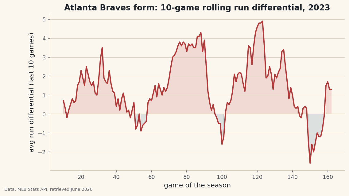
   Now the payoff. We plot the rolling differential against the game number, draw a zero line for reference, and shade above it green (playing well) and below it a contrasting color (struggling). The fill is what makes the streaks pop visually.

   fig, ax = plt.subplots(figsize=(8.6, 4.6))
   ax.axhline(0, color="#C2B7A1", linewidth=1)
   ax.plot(gl["game"], gl["roll10"], color=sdt.sport_color("baseball"), linewidth=2)
   ax.fill_between(gl["game"], gl["roll10"], 0, where=gl["roll10"] >= 0,
                   color=sdt.sport_color("baseball"), alpha=0.15)
   ax.fill_between(gl["game"], gl["roll10"], 0, where=gl["roll10"] < 0,
                   color=sdt.SPORT_COLORS["hockey"], alpha=0.15)
   ax.set_title(f"{TEAM} form: 10-game rolling run differential, 2023")
   ax.set_xlabel("game of the season")
   ax.set_ylabel("avg run differential (last 10 games)")

   

   That single line carries a whole season's narrative. Stretches where the line rides high are hot streaks; the dips are cold spells. The where= argument on fill_between is the key: it shades only the segments that satisfy the condition, so positive form gets one color and negative form another. Because the line is a 10-game average, a couple of bad games barely move it - which is exactly the noise-resistance we wanted. The flat empty start before game 10 is the rolling window filling up, just as we saw in the table.

Troubleshooting