Exponentially Weighted Averages: Form That Weights Recent Games More

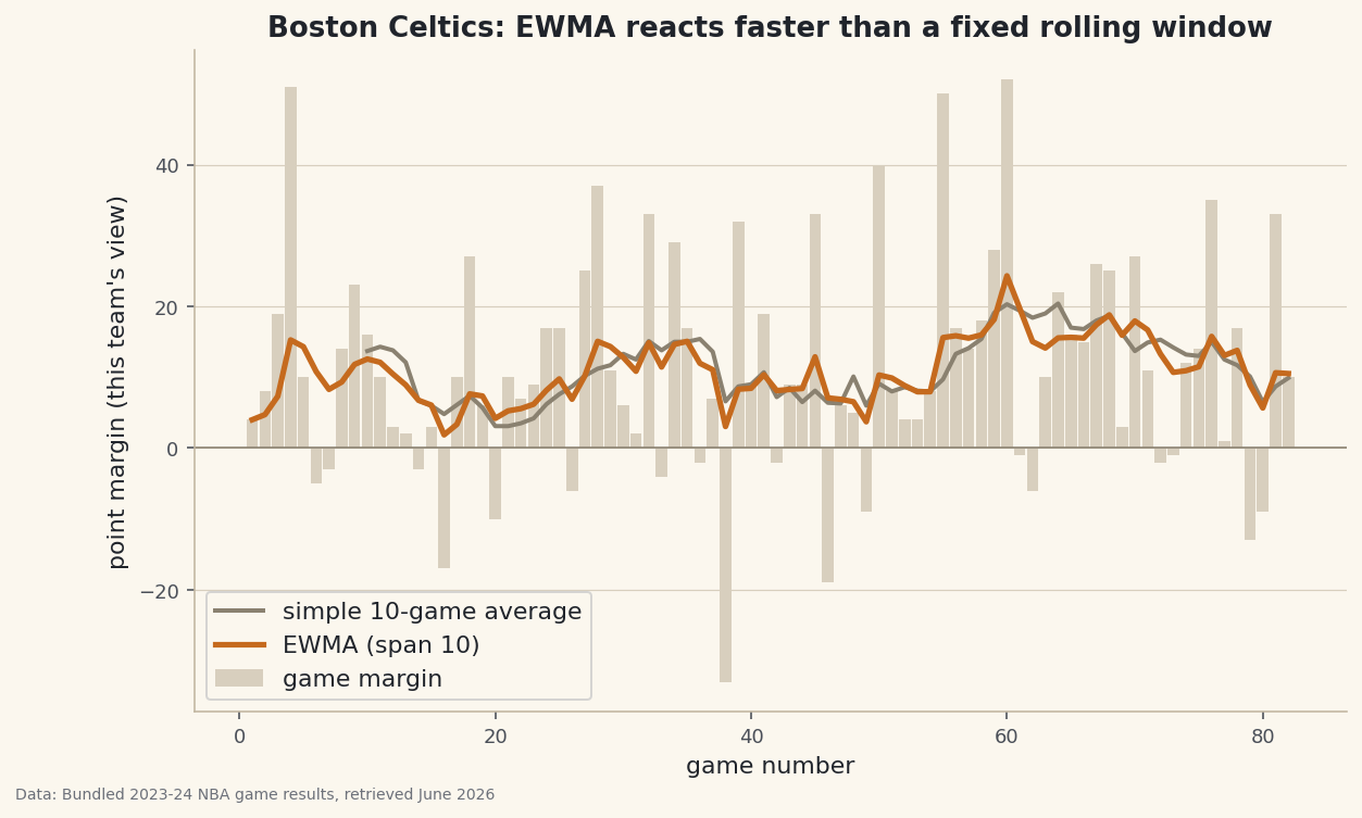
A simple 10-game rolling average has two habits worth questioning. It treats the game from three weeks ago exactly like last night's — equal weight to both — and then forgets that old game completely the instant it slides out of the window. An exponentially weighted moving average is smoother and more honest about recency: every past game still counts, but its weight decays geometrically the further back it sits. We'll take one team's game-by-game point margin, smooth it both ways, and see the EWMA react faster to a hot or cold streak without the hard edges a fixed window leaves behind.

Background, if you want it: Working with Dates, Times, and Time Series Data, from DataField.dev’s free textbook library.

This builds directly on Rolling Averages and Form (the simple-window version of the same idea) and on Summary Statistics and Distributions. The data is the bundled nba_home_results.csv (real 2023-24 games), so it runs offline.

1. Build one team's game log

   The results file stores each game once, from the home team's side. To follow a single team we have to pull both its home and away games and flip the margin so it's always from that team's point of view, then sort by date.

   import numpy as np, pandas as pd
   
   df = pd.read_csv("nba_home_results.csv"); df["date"] = pd.to_datetime(df.date)
   TEAM = "Boston Celtics"
   home = df[df.home_team == TEAM].assign(margin=lambda d: d.home_pts - d.away_pts)
   away = df[df.away_team == TEAM].assign(margin=lambda d: d.away_pts - d.home_pts)
   log = pd.concat([home[["date","margin"]], away[["date","margin"]]]) \
           .sort_values("date").reset_index(drop=True)

   Sorting by date is non-negotiable for any running average — a rolling window over shuffled games is meaningless.

2. Smooth it two ways

   The simple version is rolling(10).mean(). The exponential version is ewm(span=10, adjust=False).mean(). The span maps to a decay factor alpha = 2 / (span + 1); each new game gets weight alpha, and everything before it is discounted by (1 - alpha) per step.

   log["sma10"] = log.margin.rolling(10).mean()
   log["ewma"]  = log.margin.ewm(span=10, adjust=False).mean()
   alpha = 2 / (10 + 1)

   Where the weight actually goes

   Boston Celtics: 82 games, season margin +11.34
   EWMA span=10  ->  alpha = 2/(10+1) = 0.182
   Weight on the most recent games (newest first):
      0.182, 0.149, 0.122, 0.100, 0.081, 0.067 ...
   Last 5 games (margin | simple 10-game | EWMA):
     game 78: +17 | +11.70 | +13.79
     game 79: -13 | +10.10 |  +8.92
     game 80:  -9 |  +6.50 |  +5.66
     game 81: +33 |  +8.70 | +10.63
     game 82: +10 |  +9.90 | +10.52

   The weights are the point. With span=10, alpha is 0.182: the newest game gets 18% of the total weight, the one before it 15%, then 12%, and so on — a geometric fade that never quite reaches zero. Compare the last five games: after a +33 blowout the EWMA jumps to +10.63 while the simple average, still averaging in nine older games equally, lags at +8.70.

3. See the two curves over a season

   Plot the raw game margins as bars, then lay both smoothed lines over them. The difference in temperament is immediately visible.

   import matplotlib.pyplot as plt
   g = np.arange(1, len(log) + 1)
   fig, ax = plt.subplots()
   ax.bar(g, log.margin, color="#D8CFBE")
   ax.plot(g, log.sma10, label="simple 10-game")
   ax.plot(g, log.ewma,  label="EWMA (span 10)")
   ax.legend(); fig.savefig("ewma_vs_sma.png", dpi=144, bbox_inches="tight")

   

   The simple line is blockier — it steps whenever a big game enters or leaves the 10-game window, and it needs a full 10 games before it can report anything at all. The EWMA starts from game one and bends toward each new result, sharply after a surprise and gently once things settle. For "how good is this team right now", recency-weighting is usually the more faithful answer.

Troubleshooting