Statistical Power: How Many Games Until You Can Trust a Stat?

The bootstrap tutorial established that NBA home advantage is real: 54.3% across 1,231 games of 2023-24, whole confidence interval above 50%. Here's the uncomfortable sequel. Suppose an edge exactly that size is truly there — how many games does a significance test need before it reliably finds it? The answer is hundreds. One team's 41 home games detect it about 9% of the time; you need roughly 820 games for the standard 80%, and nearly a full league season for 90%. That detection rate is called statistical power, and once you can compute it, "we tested it and found nothing" stops sounding like "there's nothing there."

This builds directly on the permutation test — you know how to ask "is this real?"; now you'll measure when that question is even answerable — and it reuses the same bundled nba_home_results.csv, so everything runs offline. No scipy: the test's critical value comes off a simulated null, and the only formula in sight is a cross-check we build from math.erf.

1. Start from a real edge, then treat it as the truth

   Power is always computed against a hypothetical world: assume the effect is really there, at some specific size, and ask how often your test would catch it. The honest way to pick that size is to use a real one — so we take the observed 2023-24 home win rate as the true coin bias for every simulated season that follows.

   import numpy as np
   import pandas as pd
   
   games = pd.read_csv("nba_home_results.csv")
   home_win = (games["home_pts"] > games["away_pts"]).to_numpy()
   
   N_SEASON = home_win.size
   P_TRUE = home_win.mean()
   print(N_SEASON, home_win.sum(), round(P_TRUE, 4))

   The edge we'll go hunting for

   games in the bundled 2023-24 file: 1,231
   home wins: 669  ->  home win rate 0.5435 (54.3%)
   edge over a fair coin: +0.0435
   
   assume that's the TRUE home-court effect. one team's home slate is
   41 games. how often would a proper test even detect the edge there?

   A +4.35-percentage-point edge over a fair coin — the same number tutorial 64 put error bars on. Keep the size of it in your head: over 41 games, 4.35 points of win probability is less than two extra wins. That's the whole detection problem in one sentence.

2. Build the test itself: a critical value read off a simulated null

   Before we can measure a test's power we need a test. Ours is the simplest one that's still fully honest: one-sided, "do home teams win more than half?", at α = 0.05. Instead of looking up a critical value in a table, we manufacture it — simulate 100,000 fair-coin seasons at each sample size and find the smallest win count that fewer than 5% of no-edge seasons ever reach. Clear that bar and you're significant; that's the entire machine.

   rng = np.random.default_rng(84)     # fixed seed -> same numbers every run
   SIMS = 100_000
   ALPHA = 0.05
   
   def critical_wins(n, rng):
       """Smallest k with P(wins >= k | fair coin) <= ALPHA, from a simulated null."""
       null = rng.binomial(n, 0.5, size=SIMS)
       k = int(np.quantile(null, 1.0 - ALPHA))    # start near the 95th percentile
       while (null >= k).mean() > ALPHA:          # nudge up until the tail fits
           k += 1
       return k, null

   The bar you have to clear, by sample size

   one-sided test, alpha = 0.05, null = fair coin, 100,000 simulated
   seasons per sample size, seed 84
   
      n games   reject at >= wins   (win rate)   realized alpha
          41          27              0.659         0.031
         200         113              0.565         0.038
        1231         645              0.524         0.050
   
   realized alpha sits just under 0.05 because win counts are whole
   numbers - the bar lands between two integers and we take the safe side.

   Read the win-rate column: at 41 games you need a 65.9% home win rate to call the edge significant, at 200 games 56.5%, and only at 1,231 games has the bar descended to 52.4% — finally below the true 54.3%. Notice also the realized α of 0.031 at n = 41: win counts are whole numbers, the exact 5% bar lands between two integers, and taking the safe side makes the small-sample test even stricter than advertised. That detail will come back in the next step.

3. Aim the test at a world where the edge is real

   Now the actual power computation, and it's three lines: simulate 100,000 seasons where the coin truly is 54.35% home, apply the decision rule, count how often it fires. As a cross-check we run the textbook normal-approximation power formula alongside — built from math.erf, not scipy — because when a simulation and a formula built on different logic agree, you can trust both.

   import math
   
   def power_at(n, p, rng):
       """Fraction of simulated true-edge seasons the test flags as significant."""
       k, _ = critical_wins(n, rng)
       alt = rng.binomial(n, p, size=SIMS)
       return (alt >= k).mean(), k
   
   def phi(x):                              # standard normal CDF, no scipy
       return 0.5 * (1.0 + math.erf(x / math.sqrt(2.0)))
   
   def power_normal(n, p):                  # the textbook shortcut, for comparison
       c = 0.5 + 1.6449 * 0.5 / math.sqrt(n)          # reject when win rate >= c
       return 1.0 - phi((c - p) / math.sqrt(p * (1.0 - p) / n))

   Power by sample size: simulation vs formula

   true edge p = 0.5435   (the observed 2023-24 home win rate)
   
      n games   simulated power   normal approx     diff
          41        0.092            0.137        -0.046
         100        0.201            0.218        -0.017
         200        0.296            0.338        -0.042
         400        0.536            0.537        -0.001
         600        0.676            0.687        -0.011
         800        0.787            0.793        -0.006
        1000        0.862            0.866        -0.005
        1231        0.921            0.921        -0.000
        1600        0.965            0.967        -0.002
        2000        0.986            0.988        -0.001
   
   two routes, one curve: from a few hundred games up, the z-formula and
   the simulation agree to about a hundredth. at 41 games they split -
   whole-number win counts make the real test even more conservative
   than the smooth formula promises. neither route rescues small n.

   The table is the tutorial. At 41 games, power is 0.092 — a real, league-wide home edge goes undetected in more than nine of ten single-team home slates. At 400 games you're still at a coin flip (0.536). And the two columns tell a second story: from a few hundred games up they agree to about a hundredth, but at n = 41 the smooth formula says 0.137 while the truth is 0.092 — the integer-bar strictness from step 2, which the approximation can't see. The simulation isn't the lazy route here; it's the more accurate one exactly where accuracy matters.

4. Find the price of certainty, and draw the curve

   Sweep n and ask the planning questions directly: where does power reach the conventional 80%? Where 90%? This is the same arithmetic labs run before a clinical trial, pointed at a basketball argument.

   grid = np.arange(600, 1101, 10)
   power = np.array([power_at(int(n), P_TRUE, rng)[0] for n in grid])
   N80 = int(grid[np.argmax(power >= 0.80)])
   print(N80)                               # and the same sweep again for 90%

   The sample-size price list

   power at n = 41    (one team's home slate):   0.092
   power at n = 1,231 (the full league season):  0.920
   
   smallest n reaching 80% power:  ~820 games
   smallest n reaching 90% power:  ~1,160 games
   
   a true +4.4-percentage-point edge hides easily in 41 games and only
   becomes near-certain to show up across an entire league season.

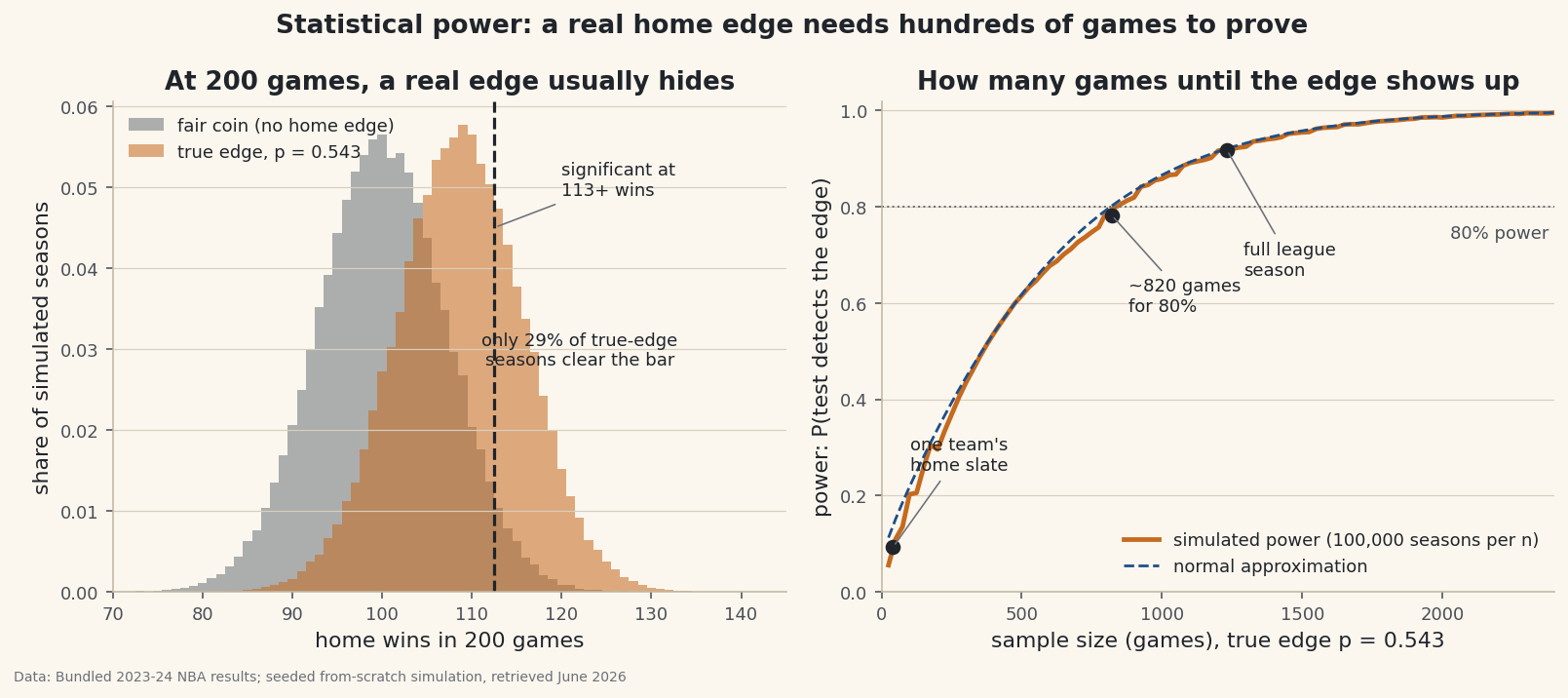
   About 820 games for 80% power, about 1,160 for 90% — and the full 1,231-game season lands at 0.920, which is why a league-wide claim tested on league-wide data works while the identical claim tested on one team's schedule is nearly hopeless. One chart holds all of it:

   import matplotlib.pyplot as plt
   
   fig, (ax1, ax2) = plt.subplots(1, 2, figsize=(11.2, 4.9))
   k, null = critical_wins(200, rng)                     # left: the overlap
   alt = rng.binomial(200, P_TRUE, size=SIMS)
   bins = np.arange(null.min(), alt.max() + 2) - 0.5
   ax1.hist(null, bins=bins, density=True, alpha=0.55, color="#6C7079")
   ax1.hist(alt,  bins=bins, density=True, alpha=0.55, color="#C56A1E")
   ax1.axvline(k - 0.5, ls="--", color="#20242B")
   
   ns = np.arange(25, 2401, 25)                          # right: the power curve
   ax2.plot(ns, [power_at(int(n), P_TRUE, rng)[0] for n in ns], color="#C56A1E")
   ax2.plot(ns, [power_normal(int(n), P_TRUE) for n in ns], ls="--", color="#1D4E89")
   ax2.axhline(0.80, ls=":", color="#6C7079")
   fig.savefig("power_curve.png", dpi=144, bbox_inches="tight")

   

   The left panel is why small samples fail: at 200 games the fair-coin world and the true-edge world overlap so much that the significance bar — placed to exclude 95% of the gray — also excludes 71% of the orange. Only 29% of seasons where the edge genuinely exists get to say so. The right panel is the remedy and its cost: the two distributions pull apart like √n, so every halving of the remaining doubt costs hundreds more games. The dotted 80% line is a convention, not a law — but crossing it at ~820 games when your dataset has 41 is a fact no convention can rescue.

What power quietly explains about sports arguments

Three things fall out of this machinery. First, "not significant" is not "no effect": at 41 games our test misses a real home edge 91% of the time, so a null result there is close to zero information — the study was incapable of finding what it looked for. Second, small-sample significance should worry you more, not less: to clear the bar at n = 41 a team needs a 65.9% home win rate, so the rare small samples that do reach significance mostly got there by overshooting the true effect — publish only those and every published edge is inflated. Third, sample size is the negotiation: before arguing about whether an effect exists, ask whether the data could have detected it. Plenty of sports debates — clutch shooting, referee bias against your team, a manager's "bad record in one-run games" — live permanently in the left half of the power curve, which is precisely why they never resolve.

Troubleshooting