Multiple Comparisons: What Survives a 30-Test Screen
Part 5 of 10 in Randomness, Inference & Simulation · course bundle (code + data)
What you'll build
The exact two-sided binomial and Fisher tests written from scratch, then run as families rather than one at a time: thirty NBA home records flag thirteen teams where an identical league flags 1.21, so Bonferroni keeps 9 and Benjamini-Hochberg keeps 12 - while the same machinery asked whether any single team has a home-court edge of its own flags five and keeps none. Closes with two shooter screens of 191 and 124 tests that land on opposite sides of the same threshold.
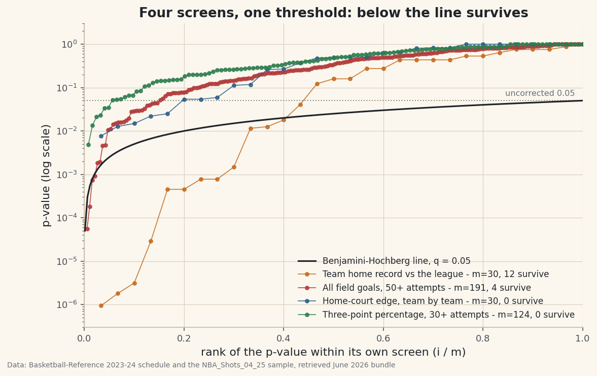
A p-value describes one question, asked once. Ask thirty questions of the same season and the arithmetic shifts underneath you without announcing itself. Here is the demonstration, run twice with opposite results. I tested all thirty NBA home records from the bundled 2023-24 season against the league’s own home-win rate, and thirteen teams came back under 0.05. A league in which every team is identical produces 1.21 such flags on average — and in 20,000 simulated seasons it never once produced thirteen — so that screen found something, and correcting it barely dents it: Bonferroni keeps 9, Benjamini-Hochberg keeps 12. Then I asked the question people actually mean by “home-court advantage” — does this team have one of its own? — with the same machinery on the same games. Five teams cleared 0.05, and not one survived any correction. Same season, same code, opposite verdicts. That is what a multiplicity correction is for. It is not a tax on your enthusiasm; it is the instrument that tells you which of those two screens you are holding.
You want the permutation test behind you for what a p-value is, and the power tutorial for why 41 games is a thin sample. Everything here runs offline from two bundled files: nba_home_results.csv (every 2023-24 game) and nba_league_shots.csv (a 25,000-shot sample of the season). No scipy — both exact tests are twelve lines of math. If you want the standard error and interval for any win count below without writing code, YalmCalc's confidence interval calculator does the proportion arithmetic in the browser.
-
One test, computed the honest way
Start with a single team so the machinery is visible. Boston went 37-4 at home. The league won 668 of 1,230 home games that season — 54.3%, after dropping the December 9 In-Season Tournament final, which was played in Las Vegas and is nobody’s home game. The exact two-sided binomial p-value is not a formula you look up; it is a sum. Compute the probability of every possible win total from 0 to 41, then add up the ones no more likely than what you saw. Work in logs with
lgammaso the binomial coefficient never overflows.python import math import pandas as pd def log_pmf(k, n, p): return (math.lgamma(n + 1) - math.lgamma(k + 1) - math.lgamma(n - k + 1) + k * math.log(p) + (n - k) * math.log1p(-p)) def binom_test(k, n, p): """Exact two-sided p: every outcome at least as unlikely as this one.""" obs = log_pmf(k, n, p) + 1e-9 return min(1.0, sum(math.exp(log_pmf(i, n, p)) for i in range(n + 1) if log_pmf(i, n, p) <= obs)) games = pd.read_csv("nba_home_results.csv") season = games[games.date != "2023-12-09"].copy() # neutral-site final season["home_win"] = (season.home_pts > season.away_pts).astype(int) p_home = season.home_win.mean() bos = season[season.home_team == "Boston Celtics"] k, n = int(bos.home_win.sum()), len(bos) print(f"league {100 * p_home:.1f}% at home; Boston {k}-{n - k}") print("exact two-sided p =", binom_test(k, n, p_home))One team, one test: Boston's home record against the league's home-win rate1231 rows; dropping the 2023-12-09 neutral-site final leaves 1230 home games home teams won 668 of 1230 = 54.3% <- the benchmark every team is tested against Boston went 37-4 at home (90.2%) P(exactly 37 of 41 at 0.5431) = 6.840e-07 outcomes at least that unlikely: 12 of the 42 possible totals exact two-sided p = 9.44e-07
Boston’s 37 wins in 41 home games has a probability of 6.84 in ten million on its own, and 12 of the 42 possible win totals are at least that unlikely, which sums to an exact two-sided p of 9.44 × 10⁻⁷. Taken alone that is about as decisive as a single season can be. The trouble starts on the next line of code, where I do it twenty-nine more times.
-
Run it thirty times and count the winners
The same test, once per home team, sorted by p-value. Nothing about any individual test has changed — each one is still correct — and that is precisely the problem, because the thing being reported is no longer any individual test. It is the smallest of thirty.
python rows = [] for team, sub in season.groupby("home_team"): n, k = len(sub), int(sub.home_win.sum()) rows.append((team, n, k, 100 * k / n, binom_test(k, n, p_home))) screen = pd.DataFrame(rows, columns=["team", "games", "wins", "win_pct", "p"]) screen = screen.sort_values("p").reset_index(drop=True) m = len(screen) print(screen.head(10).to_string(index=False)) print(f"{(screen.p < 0.05).sum()} of {m} under 0.05; " f"{m * 0.05:.1f} expected by chance alone")Thirty tests, thirteen flags - against 1.5 expected if nothing were going onthe same test, run 30 times - once per home team team games wins win_pct p Boston Celtics 41 37 90.2 9.44e-07 Washington Wizards 41 7 17.1 1.80e-06 Detroit Pistons 40 7 17.5 3.15e-06 Memphis Grizzlies 41 9 22.0 2.91e-05 Portland Trail Blazers 41 11 26.8 4.51e-04 Charlotte Hornets 41 11 26.8 4.51e-04 Denver Nuggets 41 33 80.5 7.74e-04 Oklahoma City Thunder 41 33 80.5 7.74e-04 San Antonio Spurs 41 12 29.3 1.48e-03 Toronto Raptors 41 14 34.1 1.15e-02 ... 13 of 30 teams come in under p < 0.05 tests expected under 0.05 by chance alone: 1.5Thirteen of thirty. Written up carelessly that becomes “43% of NBA teams had a statistically significant home record,” a sentence that is true, useless, and misleading in the same breath. Note also what this screen is actually measuring: Boston is at the top because Boston won 64 games, and Washington is second because Washington won 15. Team quality and home court are tangled here in exactly the way an aggregated split tangles them. I untangle it in step 5. First, the count needs a null.
-
What a league with nothing going on produces
The textbook line is that at α = 0.05 with m independent tests, the chance of at least one false alarm is 1 − 0.95m, which at m = 30 is 78.5%. Do not take that on trust when you can build the league yourself. Simulate 20,000 seasons in which all thirty teams are identical — every home game an independent 54.3% coin — and run the identical screen on each one. Because each team’s home games are a disjoint set of games, the thirty tests here really are independent, which is exactly the condition the formula needs.
python import numpy as np rng = np.random.default_rng(93) sizes = screen.games.to_numpy() lut = {int(n): np.array([binom_test(k, int(n), p_home) for k in range(int(n) + 1)]) for n in np.unique(sizes)} # p-value lookup per (n, k) draws = rng.binomial(sizes, p_home, size=(20000, m)) sim_p = np.empty(draws.shape, dtype=float) for j, n in enumerate(sizes): sim_p[:, j] = lut[int(n)][draws[:, j]] hits = (sim_p < 0.05).sum(axis=1) print("average flags per season:", round(hits.mean(), 2)) print("seasons flagging at least one:", f"{100 * (hits >= 1).mean():.1f}%", " vs 1 - 0.95**30 =", f"{100 * (1 - 0.95 ** 30):.1f}%") print("seasons flagging 13 or more:", int((hits >= 13).sum()))20,000 identical leagues: 1.21 flags on average, 71.1% flag somebody, never thirteen20000 simulated seasons in which all 30 teams are identical (every home game an independent 54.3% coin) average teams flagged at p < 0.05 : 1.21 seasons flagging at least one team : 71.1% what 1 - 0.95^30 predicts : 78.5% seasons flagging three or more : 12.0% seasons flagging 13 or more (as we saw) : 0 of 20000 busiest simulated season : 7 flags flags per season: 0: 5781 1: 7312 2: 4503 3: 1782 4: 504 5: 100An empty league flags 1.21 teams per season on average and flags at least one in 71.1% of seasons. Three or more happens 12.0% of the time. Thirteen happened 0 times in 20,000, and the busiest simulated season managed seven. So the screen is real: whatever else is true, these thirty home records are not thirty draws from one distribution. Two footnotes worth keeping. First, 71.1% is meaningfully below the textbook 78.5%, and the reason is discreteness — an exact test on 41 games can only take 42 distinct p-values, none of which lands on 0.05, so the rule “reject below 0.05” actually rejects less often than 5% of the time. Exact tests are conservative, and every correction below inherits that conservatism. Second, this is the same trick as the Monte Carlo season: when you cannot reason about a null, build it.
-
Bonferroni for the family, Benjamini-Hochberg for the discoveries
The two standard corrections answer two different questions. Bonferroni controls the family-wise error rate — the chance of even one false rejection — by testing each hypothesis at α/m. Benjamini and Hochberg control the false discovery rate: of the hypotheses you end up rejecting, the expected share that are false. BH sorts the p-values, compares the i-th smallest against (i/m) × q, and rejects everything up to the largest i that passes — that last part is the step people get wrong.
python import numpy as np def bh_survivors(pvals, q): p = np.sort(np.asarray(pvals, dtype=float)) m = len(p) below = np.nonzero(p <= (np.arange(1, m + 1) / m) * q)[0] return int(below.max() + 1) if len(below) else 0 alpha = 0.05 ladder = screen.head(16).copy() ladder["i"] = np.arange(1, len(ladder) + 1) ladder["bh_crit"] = ladder["i"] / m * alpha ladder["passes"] = np.where(ladder.p <= ladder.bh_crit, "yes", "no") print(ladder[["i", "team", "p", "bh_crit", "passes"]].to_string(index=False)) print("Bonferroni cut", alpha / m, "->", int((screen.p < alpha / m).sum()), "survive") print("BH q=0.05 ->", bh_survivors(screen.p, alpha), " BH q=0.10 ->", bh_survivors(screen.p, 0.10))The BH ladder: rank 12 clears its step at 0.0200, rank 13 misses at 0.0217m = 30 tests at alpha = 0.05 Bonferroni: reject when p < alpha/m = 0.001667 -> 9 survive Benjamini-Hochberg: reject when p <= (i/m) x q -> 12 survive i team p bh_crit passes 1 Boston Celtics 9.44e-07 0.00167 yes 2 Washington Wizards 1.80e-06 0.00333 yes 3 Detroit Pistons 3.15e-06 0.00500 yes 4 Memphis Grizzlies 2.91e-05 0.00667 yes 5 Portland Trail Blazers 4.51e-04 0.00833 yes 6 Charlotte Hornets 4.51e-04 0.01000 yes 7 Denver Nuggets 7.74e-04 0.01167 yes 8 Oklahoma City Thunder 7.74e-04 0.01333 yes 9 San Antonio Spurs 1.48e-03 0.01500 yes 10 Toronto Raptors 1.15e-02 0.01667 yes 11 Milwaukee Bucks 1.26e-02 0.01833 yes 12 Minnesota Timberwolves 1.79e-02 0.02000 yes 13 Orlando Magic 4.09e-02 0.02167 no 14 Los Angeles Lakers 1.22e-01 0.02333 no 15 Houston Rockets 1.59e-01 0.02500 no 16 New York Knicks 1.59e-01 0.02667 no largest i whose p clears its own step: 12 -> reject ranks 1..12 uncorrected 13 BH(q=0.05) 12 BH(q=0.10) 13 Bonferroni 9
Bonferroni’s threshold is 0.05/30 = 0.001667, and nine teams clear it — through San Antonio at 0.00148, stopping before Toronto at 0.0115. BH is looser and the arithmetic is worth reading line by line: Minnesota sits at rank 12 with p = 0.0179 against a step of 12/30 × 0.05 = 0.0200, so it passes; Orlando sits at rank 13 with p = 0.0409 against 0.02167, so it fails; twelve is the largest passing rank, so ranks 1 through 12 are all rejected. Raise q to 0.10 and Orlando’s step becomes 0.0433, it clears, and the count goes to 13. The promises differ as much as the counts do. Bonferroni says there is at most a 5% chance that even one of its nine is spurious. BH says that among its twelve, roughly 5% — call it one team in twenty, so probably none here — is expected to be a false discovery. Neither is stricter in the abstract; they insure against different accidents.
-
The same machinery, the opposite verdict
Now the question people actually mean. Instead of asking whether a team’s home record beats the league, ask whether it beats its own road record — which cancels team quality, because the same team plays both halves. That is a 2×2 table per team, so the test is Fisher’s exact rather than the binomial, but the multiplicity arithmetic is identical: thirty tests, one family.
python def fisher_exact(a, b, c, d): """Exact two-sided p for [[a, b], [c, d]] - hypergeometric, no scipy.""" n, r1, r2, c1 = a + b + c + d, a + b, c + d, a + c prob = lambda x: math.comb(r1, x) * math.comb(r2, c1 - x) / math.comb(n, c1) obs = prob(a) * (1 + 1e-9) return min(1.0, sum(prob(x) for x in range(max(0, c1 - r2), min(r1, c1) + 1) if prob(x) <= obs)) rows = [] for team in sorted(season.home_team.unique()): h = season[season.home_team == team] a = season[season.away_team == team] hw = int(h.home_win.sum()) aw = int((a.away_pts > a.home_pts).sum()) rows.append((team, hw, len(h) - hw, aw, len(a) - aw, 100 * (hw / len(h) - aw / len(a)), fisher_exact(hw, len(h) - hw, aw, len(a) - aw))) hca = pd.DataFrame(rows, columns=["team", "hw", "hl", "aw", "al", "gap_pp", "p"]) hca = hca.sort_values("p").reset_index(drop=True) print(hca.head(8).to_string(index=False)) print("raw", int((hca.p < 0.05).sum()), " Bonferroni", int((hca.p < 0.05 / m).sum()), " BH(0.05)", bh_survivors(hca.p, 0.05), " BH(0.10)", bh_survivors(hca.p, 0.10)) print("pooled over all games:", binom_test(int(season.home_win.sum()), len(season), 0.5))Screen two: five raw flags, zero survivors, and a pooled effect that is unmistakablescreen 2: does THIS team have a home-court advantage of its own? (exact 2x2 test of each team's home record against its own road record) team hw hl aw al gap_pp p Houston Rockets 27 14 14 27 +31.7 0.0077 Milwaukee Bucks 31 11 18 22 +28.8 0.0128 Boston Celtics 37 4 27 14 +24.4 0.0148 Utah Jazz 21 20 10 31 +26.8 0.0220 Orlando Magic 29 12 18 23 +26.8 0.0249 Oklahoma City Thunder 33 8 24 17 +22.0 0.0538 Denver Nuggets 33 8 24 17 +22.0 0.0538 Memphis Grizzlies 9 32 18 23 -22.0 0.0591 ... teams with a positive home-road gap: 23 of 30 uncorrected p < 0.05: 5 Bonferroni: 0 BH(q=0.05): 0 BH(q=0.10): 0 league-wide, pooled over all 1230 games: 668-562, exact p = 0.0027 4000 simulated leagues where every team shares the SAME home edge: teams flagged, average 2.84; 5 or more happened 14.7% of the timeTwenty-three of thirty teams have a positive home-road gap and six are negative (Dallas went 25-16 both ways, to the game). Houston has the largest gap in the league at +31.7 points and the smallest p-value at 0.0077. Five teams clear an uncorrected 0.05. Zero survive Bonferroni, and zero survive BH at q = 0.05 or even q = 0.10 — the first BH step is 0.05/30 = 0.00167 and Houston misses it by a factor of 4.6. And to be sure five raw flags is not itself a signal, I simulated 4,000 leagues in which every team shares the same home edge: the average was 2.84 flags, and five or more turned up 14.7% of the time. Five is ordinary. Meanwhile the pooled test over all 1,230 games — one hypothesis, specified in advance, nothing to correct — gives 668-562 at p = 0.0027. That is the honest summary: home advantage is a fact about the league and a rumor about any particular team. It is the same gap the five-league comparison measures with everything pooled, and 41 home games per team is simply not enough to attribute it, exactly as the power tutorial warned.
-
Scale it: 191 tests, then 124
Thirty tests is a small family. Screens in practice run to hundreds, so take the 25,000-shot sample and test every shooter with at least 50 attempts against the league’s field-goal percentage — 191 tests — then repeat on three-pointers only, 30 attempts and up, 124 tests. Two screens, same code, and they land on opposite sides of the line.
python shots = pd.read_csv("nba_league_shots.csv") lg_fg = shots.SHOT_MADE.mean() def screen_shooters(frame, floor, base): t = frame.groupby("PLAYER_NAME").SHOT_MADE.agg(att="size", made="sum") t = t[t.att >= floor].copy() t["pct"] = 100 * t.made / t.att t["p"] = [binom_test(int(k), int(n), base) for n, k in zip(t.att, t.made)] return t.sort_values("p") fg = screen_shooters(shots, 50, lg_fg) threes = shots[shots.SHOT_TYPE == "3PT Field Goal"] tp = screen_shooters(threes, 30, threes.SHOT_MADE.mean()) for name, t in [("all field goals", fg), ("threes only", tp)]: mm = len(t) print(f"{name}: m={mm} raw {int((t.p < 0.05).sum())} " f"expected {mm * 0.05:.1f} Bonferroni {int((t.p < 0.05 / mm).sum())} " f"BH(0.05) {bh_survivors(t.p, 0.05)}") print(t.head(4).to_string())191 shooters: 28 flags against 9.6 expected. 124 three-point shooters: 6 against 6.225000 shots, 547 shooters; league 47.2% from the field, 36.5% from three all field goals, 50+ attempts: m = 191 tests against 47.2% p < 0.05 uncorrected 28 expected by chance 9.6 Bonferroni 2 BH(q=0.05) 4 BH(q=0.10) 6 att made pct p PLAYER_NAME Nikola Jokic 169 106 62.7 0.0001 Nic Claxton 62 44 71.0 0.0002 Scoot Henderson 86 25 29.1 0.0007 Giannis Antetokounmpo 170 102 60.0 0.0009 threes only, 30+ attempts: m = 124 tests against 36.5% p < 0.05 uncorrected 6 expected by chance 6.2 Bonferroni 0 BH(q=0.05) 0 BH(q=0.10) 0 att made pct p PLAYER_NAME Stephen Curry 108 54 50.0 0.0049 Grayson Allen 52 28 53.8 0.0135 Jaden McDaniels 35 6 17.1 0.0210 Duncan Robinson 54 28 51.9 0.0233 league shot diet: 29.5% of shots from the restricted area the four field-goal survivors, by diet: Nikola Jokic 40.8% restricted area Nic Claxton 77.4% restricted area Scoot Henderson 33.7% restricted area Giannis Antetokounmpo 61.8% restricted areaThe field-goal screen flags 28 shooters against 9.6 expected; two clear Bonferroni, four clear BH at q = 0.05 and six at q = 0.10. The three-point screen flags 6 against 6.2 expected, and nothing survives either correction — Stephen Curry, at 50.0% on 108 attempts, has the smallest p-value in the family at 0.0049 and needs 0.0004 to clear the first BH step. Then read the four field-goal survivors and notice what the screen actually caught. The league takes 29.5% of its shots from the restricted area; Nikola Jokic takes 40.8%, Giannis Antetokounmpo 61.8%, Nic Claxton 77.4%. A screen on raw field-goal percentage finds shot diet and finishing at the same time and cannot tell you which. The fourth survivor makes that concrete from the other end: Scoot Henderson also shoots nearer the rim than the league does, at 33.7%, and still converts 29.1% — the worst mark in the screen. The three-point screen has no diet confound left to find, and finds nothing, because 108 attempts is what a 25,000-shot sample gives its busiest shooter. That is a statement about the sample, not about Curry.
Data: Bundled (Basketball-Reference 2023-24 results and a 25,000-shot sample of the public NBA_Shots_04_25 log), retrieved June 2026 bundle (complete 2023-24 season)
Where this stops working
Six limits, in the order they would bite. First, the benchmark is estimated from the same games it judges: the 54.3% league rate is computed from the 1,230 home games the thirty tests then partition, so the thirty results are not free of each other in aggregate — the deviations must sum to zero. Second, independence is a property you have to check, not assume. It holds for the thirty home-record tests, whose games are disjoint, which is why 1 − 0.9530 was the right formula to compare against. It does not hold for the shooter screens: teammates share possessions, defenses and lineups. BH is proved to control the FDR under positive dependence; when the dependence structure is unknown, the Benjamini-Yekutieli variant divides q by the harmonic sum (5.83 at m = 191) and holds under any dependence at a real cost in power. Third, discreteness makes every exact test conservative, so the true size of these screens is below the nominal 0.05 and the corrections are stricter than advertised. Fourth, correction does not rescue a small sample: 25 teams failing to reject in step 5 is not evidence they lack a home edge, it is evidence that 41 home games cannot see one. Fifth, the field-goal screen conflates diet with skill, and no amount of p-value adjustment fixes a badly posed hypothesis. Sixth, a screen selects hypotheses with the same data it tests them on, so the surviving effect sizes are biased away from the mean — Houston’s +31.7 points is the largest of thirty draws and should be shrunk before anyone forecasts with it, for the reasons the regression tutorial lays out in full.
Sources. Game results: Basketball-Reference 2023-24 schedule pages, bundled by the site’s build script. Shots: the public NBA_Shots_04_25 shot log, 2023-24 season, a 25,000-row sample. The false discovery rate and the step-up procedure used here: Yoav Benjamini and Yosef Hochberg, “Controlling the False Discovery Rate: A Practical and Powerful Approach to Multiple Testing,” Journal of the Royal Statistical Society, Series B 57(1), 1995, doi:10.1111/j.2517-6161.1995.tb02031.x; the dependence-proof variant is Benjamini and Yekutieli, The Annals of Statistics 29(4), 2001, doi:10.1214/aos/1013699998. The α/m correction as it is used in practice comes from Olive Jean Dunn, “Multiple Comparisons Among Means,” Journal of the American Statistical Association 56(293), 1961, doi:10.1080/01621459.1961.10482090. Every count on this page is recomputed by the tutorial’s script, which carries 73 assertions and fails rather than printing a number it cannot reproduce.
Troubleshooting
My p-values differ from these in the third decimal
Almost certainly a two-sided convention, not a bug. There are two common definitions: the one used here sums the probability of every outcome at least as unlikely as the observed one, and the other doubles the smaller one-sided tail. They agree when the null probability is 0.5 and diverge when it is not — and 0.543 is not. R’s binom.test and scipy’s binomtest both default to the first. If you are comparing against a normal approximation instead, expect much larger gaps in the tails, which is where this whole exercise lives.
BH kept a hypothesis but dropped one with a smaller p-value
You applied the comparison pointwise. BH is a step-up procedure: find the largest rank i whose p-value clears (i/m) × q, then reject everything from rank 1 to i, including ranks that failed their own step on the way. Orlando at rank 13 fails its step of 0.02167, so the answer is 12 — but had rank 13 passed, ranks that individually failed below it would still have been rejected. Sorting the p-values first and taking below.max() + 1 is the whole implementation.
OverflowError or math domain error in the binomial
You are computing math.comb(n, k) * p ** k directly. The coefficient is an exact integer that outgrows a float long before n gets interesting, while p ** k underflows toward zero from the other side. Do it in log space with lgamma, as above, and exponentiate once at the end. The domain error is the other classic: math.log(p) with p = 0 or 1, which happens the moment you feed the function a base rate computed from an empty slice.
Challenge yourself
Three extensions, each a few lines. First, drop the attempt floor in the field-goal screen from 50 to 25 and watch m climb past 300 while the BH survivor list barely moves — more tests bought you more noise and no discoveries, which is the argument for setting a floor before you look. Second, implement Benjamini-Yekutieli by dividing q by the harmonic sum of 1 to m and report how many of the four field-goal survivors are left once you stop assuming independence. Third, the honest stability check: split the season into halves by date, rerun the thirty-team screen on each half, and count how many of the thirteen raw flags appear in both. A correction is a guess about replication; that experiment is the thing itself.
Download the script
The full script, ready to run - the finished script that generated every figure on this page.
Download the finished script (93_multiple_comparisons_bonferroni_and_fdr.py)This script imports a small shared helper (and reads any bundled sample data) that live next to it in /downloads/ — grab these into the same folder so it runs as-is: sdt_common.py, sdt_nba.py. Or skip the collecting: the Randomness, Inference & Simulation bundle has this whole course’s scripts and data in one ZIP.