Simpson's Paradox: When Every Split Disagrees With the Total

Buried in the bundled file of 25,000 real NBA shots is a fact that sounds impossible: Lauri Markkanen hit a higher percentage of his two-pointers than Shai Gilgeous-Alexander, a higher percentage of his three-pointers — and a lower percentage of his shots overall. No typo, no rounding trick, no missing data. Every split says one thing and the total says the other, and both are computed correctly from the same table. That's Simpson's paradox, the most famous trap in aggregated data, and this tutorial doesn't construct a toy example of it — it finds a real one by scanning the data, opens up the arithmetic that causes it, and then shows it isn't even rare.

The only tools are groupby skills and a clear head: no scipy, no randomness, every number deterministic and re-runnable offline. What you take away is a data-literacy reflex — whenever two groups are compared on a rate, ask what happens when you split — that will save you from published nonsense more often than any significance test.

1. Ask the aggregate: who's the better shooter?

   Start the way every argument starts — with the headline number. Overall field-goal percentage: makes divided by attempts, all shots pooled. The bundled file has 547 players; we pull two stars out of it.

   import pandas as pd
   
   shots = pd.read_csv("nba_league_shots.csv")
   A, B = "Lauri Markkanen", "Shai Gilgeous-Alexander"
   pair = shots[shots["PLAYER_NAME"].isin([A, B])]
   
   overall = (pair.groupby("PLAYER_NAME")["SHOT_MADE"]
                  .agg(made="sum", attempts="count", fg_pct="mean"))
   print(overall.sort_values("fg_pct", ascending=False))

   The aggregate verdict

   25,000 shots, 547 players in the bundled file
   
                            made  attempts  fg_pct
   PLAYER_NAME                                    
   Shai Gilgeous-Alexander    90       174   0.517
   Lauri Markkanen            57       112   0.509
   
   overall field goal %: Shai Gilgeous-Alexander ahead by +0.008

   Gilgeous-Alexander, by eight thousandths: 0.517 to 0.509. Small, but the direction is clear, the arithmetic is correct, and this is exactly the kind of number that ends a bar argument. Hold that verdict — it's about to lose an argument with its own ingredients. (One note for honesty: this file is a 25,000-shot sample of a season, so these are the sample's percentages, not the players' full official season lines. The paradox we're about to expose is a property of the table itself — it would be just as real in any table shaped like this.)

2. Split by shot type and watch the verdict flip

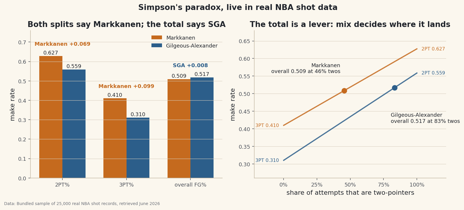
   Now the one extra groupby key that every rate comparison deserves. Two-pointers and three-pointers are different jobs, so grade them separately:

   split = (pair.groupby(["SHOT_TYPE", "PLAYER_NAME"])["SHOT_MADE"]
                .agg(made="sum", attempts="count", fg_pct="mean"))
   print(split.round(3))

   The same shots, disaggregated

                                           made  attempts  fg_pct
   SHOT_TYPE      PLAYER_NAME                                    
   2PT Field Goal Lauri Markkanen            32        51   0.627
                  Shai Gilgeous-Alexander    81       145   0.559
   3PT Field Goal Lauri Markkanen            25        61   0.410
                  Shai Gilgeous-Alexander     9        29   0.310
   
   2PT Field Goal: Lauri Markkanen ahead by +0.069
   
   3PT Field Goal: Lauri Markkanen ahead by +0.099
   
   Lauri Markkanen shoots better on twos AND on threes - yet trails overall.
   that is Simpson's paradox, and every number above is real.

   Markkanen wins the twos by +6.9 points (0.627 vs 0.559) and the threes by +9.9 points (0.410 vs 0.310) — and still trails the total. Sit with that for a second, because your brain wants to reject it: there is no shot in the file where Markkanen's category percentage isn't higher, yet pooling the very same rows reverses the sign. Nothing was miscounted. The total is simply answering a different question than the splits are, and step 3 shows exactly which one.

3. Open the machine: a total is a mix-weighted average

   An overall percentage is not a fact about shooting skill alone — it's a weighted average of the split percentages, weighted by how often each player takes each kind of shot. Write that identity out and the paradox stops being spooky:

   mix = (pair.groupby(["PLAYER_NAME", "SHOT_TYPE"])["SHOT_MADE"].count()
              .groupby(level=0).transform(lambda s: s / s.sum())
              .unstack())
   print(mix.round(3))
   # overall = share_2pt * fg2_pct  +  share_3pt * fg3_pct   (exactly)

   The weighted average, computed by hand

   share of each player's attempts by shot type:
   
   SHOT_TYPE                2PT Field Goal  3PT Field Goal
   PLAYER_NAME                                            
   Lauri Markkanen                   0.455           0.545
   Shai Gilgeous-Alexander           0.833           0.167
   
   overall = (share of twos) x (2PT%) + (share of threes) x (3PT%):
   
     Lauri Markkanen          0.455 x 0.627 + 0.545 x 0.410 = 0.509
     Shai Gilgeous-Alexander  0.833 x 0.559 + 0.167 x 0.310 = 0.517
   
   twos are simply the easier shot class: league-wide in this file,
   54.1% of two-pointers go in vs 36.5% of threes.
   
   the hidden confounder is the mix: Shai takes 83% of his
   shots as (easier) twos; Lauri takes 54% as threes. the
   aggregate rewards the shot diet, not the shooting.

   There's the hidden third variable: shot mix. League-wide in this file, 54.1% of twos go in against 36.5% of threes — twos are just the easier class. Gilgeous-Alexander takes 83% of his shots from the easy class; Markkanen takes 54% of his from the hard one. So SGA's overall sits close to his (good) two-point rate, while Markkanen's is dragged toward his (necessarily lower) three-point rate. The aggregate isn't lying about the arithmetic — it's silently grading shot diet along with shot making, and the diets are wildly unbalanced. That's the general anatomy of Simpson's paradox: a lurking group variable, unequal group sizes across the things being compared, and a rate that differs between groups. Whenever those three line up, the total and the splits are free to disagree.

4. Scan every pair: this is a hazard, not a freak

   One cherry-picked pair proves nothing about how often this bites. So don't cherry-pick — scan. Take every player with at least 100 shots and at least 15 attempts of each type, and test every pair in both directions for a full reversal: better on both splits, worse overall.

   import itertools
   
   reversals = []
   for a, b in itertools.combinations(eligible, 2):
       for x, y in ((a, b), (b, a)):
           wins_both = (fg2[x] > fg2[y]) and (fg3[x] > fg3[y])
           if wins_both and fg_all[x] < fg_all[y]:
               reversals.append((x, y))
   print(len(reversals))

   Every high-volume pair, tested

   players with >= 100 shots and >= 15 attempts of each type: 71
   pairs scanned: 2,485
   Simpson reversals found: 53 (2.1% of pairs)
   
   strongest five (by the smaller of the two split gaps):
     Lauri Markkanen beats Shai Gilgeous-Alexander on both splits (weaker gap +0.069) yet trails overall
     Lauri Markkanen beats Brandon Ingram on both splits (weaker gap +0.068) yet trails overall
     Jordan Poole beats Brandon Ingram on both splits (weaker gap +0.056) yet trails overall
     Luka Doncic beats Nikola Vucevic on both splits (weaker gap +0.055) yet trails overall
     Jayson Tatum beats Nikola Vucevic on both splits (weaker gap +0.052) yet trails overall
   
   the featured pair is #1 of 53 - the strongest reversal
   in the file, found by exhaustive scan, not construction.

   53 reversals in 2,485 pairs — about one comparison in fifty, sitting in a single season's shot sample, using the crudest possible split. And the pair we featured is the strongest of the 53, found by exhaustive search rather than construction. One chart holds the whole tutorial:

   fig, (ax1, ax2) = plt.subplots(1, 2, figsize=(11.2, 4.9))
   ax1.bar(...)                    # left: 2PT%, 3PT%, overall, side by side
   for p in (A, B):                # right: overall = a point on the mix line
       ax2.plot([0, 1], [fg3[p], fg2[p]])          # 3PT% at x=0, 2PT% at x=1
       ax2.scatter([share_2pt[p]], [fg_all[p]])    # the total, placed by mix
   fig.savefig("reversal.png", dpi=144, bbox_inches="tight")

   

   The right panel is the one to internalize. Each player's overall percentage is a dot on a line running from his three-point rate to his two-point rate, placed by his share of two-point attempts. Markkanen's line sits above SGA's line everywhere — that's "better at both" — but his dot sits at 46% twos while SGA's sits at 83%, and position on the lever beats height of the lever. An aggregate is a dot; the skill is the line. Compare dots and you're partly comparing where they sit, whether you meant to or not.

So which number is right — the split or the total?

Neither is wrong; they answer different questions, and the discipline is matching the number to the question. If the question is "who is more likely to make a given shot?" — you're choosing who takes a catch-and-shoot three — the split is the answer and the aggregate is actively misleading, because the mix is a nuisance variable you never meant to grade. If the question is "whose actual shot diet produced more makes per attempt?", the aggregate answers it honestly — but notice how rarely that's the real question, and in basketball raw FG% is the wrong currency anyway, since a made three is worth half again a made two (that's the effective field-goal fix in the challenge). The general rule: when the group mix is a choice you intend to credit, the aggregate has a case; when the mix is a confounder, split. This same reversal has decided real arguments for fifty years — the canonical 1973 Berkeley admissions study, where the aggregate suggested bias that mostly vanished department by department, and the textbook baseball case where David Justice out-hit Derek Jeter in both 1995 and 1996 while Jeter out-hit him combined. Sports is unusually rich soil for it because exposure is never balanced: platoon splits, home/away schedules, garbage time, shot zones, pitcher handedness. Any time two rates are compared across different exposure mixes, check the split before you believe the total.

Troubleshooting