Is xG Calibrated? Checking a Published Model Against 1,494 Real Shots

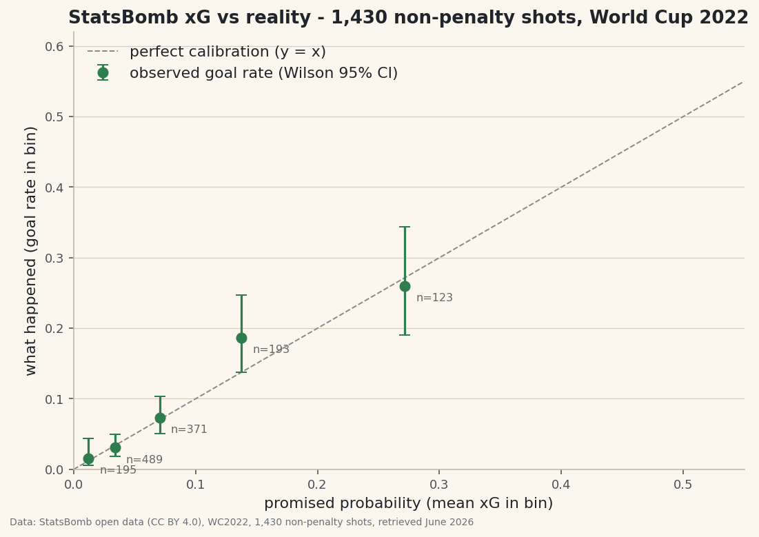
Every xG value is a promise: “shots like this one go in about this often.” You have drawn those promises on a pitch and summed them into a table — this tutorial finally asks whether they are true. The audit runs on StatsBomb’s own xG for all 1,494 shots of the 2022 World Cup, and it comes back more interesting than a yes: the tournament scored 14 goals more than its non-penalty xG said it should — and that surplus is still only 1.4 standard errors from the model’s promise, which is the real lesson. In five of six probability bins the observed goal rate sits inside a 95% interval of the promise, the model beats a know-nothing baseline by 19.8% on Brier score, and the one bin that misses does so by a rounding error’s width. Calibration checking is not a verdict machine; it is the discipline of knowing how loudly one tournament can speak.

You need groupby fluency and it helps to have met interval thinking in the statistics course. Everything runs offline from the bundled wc2022_shots.csv — one row per shot, every match of the tournament. Data provided by StatsBomb open data (CC BY 4.0); the xG column is their model’s, which is exactly the point — we are auditing a published model, not our own homework.

1. Know what a row is before you average it

   Load the file and count goals: 195. The 2022 World Cup did not have 195 shot-scored goals in play, and the difference is the whole first step. Group by period and period 5 confesses: 41 rows are penalty-shootout kicks, each carrying an xG value and 26 of them “goals,” none of which appear in any match score. And the mirror-image trap: own goals are nobody’s shot, so they are not in a shot table at all — a shot file can never reconcile to the official goal count by itself. Every calibration mistake downstream of this step would be baked in silently.

   import pandas as pd
   
   shots = pd.read_csv("wc2022_shots.csv")
   print(len(shots), "shots,", shots.is_goal.sum(), "rows flagged as goals")
   print(shots.groupby("period").agg(rows=("xg", "size"), goals=("is_goal", "sum"),
                                     penalties=("is_penalty", "sum")))
   
   match = shots[shots.period < 5]          # real match play only
   open_sp = match[match.is_penalty == 0]    # non-penalty match shots

   1,494 rows; period 5 is the shoot-outs, and own goals are never here at all

   1494 shots, 195 rows flagged as goals
   
   by period (5 = penalty shoot-outs):
      period  rows  goals  penalties
   0       1   607     66         12
   1       2   801     99         10
   2       3    20      1          0
   3       4    25      3          1
   4       5    41     26         41
   
   shoot-out rows: 41, 'goals' among them: 26 - none of which appear in a match score
   own goals: not shots, so never in this table at all

2. Calibration in the large — and how loudly one tournament can speak

   If the model is honest, summed xG should land near actual goals. Each shot is a Bernoulli trial with its own probability, so the promise comes with a standard error of sqrt(sum p(1-p)) — about ±10 goals for this tournament. The non-penalty ledger reads 137.9 promised, 152 delivered: +14.1, a 10% hot streak… at z = +1.39. You cannot convict a model on that. In-game penalties, priced at 0.783 each, delivered 17 of a promised 18 — on the nose. And the naive read that keeps the shoot-outs in (188 xG vs 195 “goals”) looks like the closest match of all while being built from rows that are not match goals: agreement you get by averaging garbage is still garbage.

   import numpy as np
   
   for name, df in [("non-penalty match shots", open_sp),
                    ("in-game penalties", match[match.is_penalty == 1]),
                    ("all match shots", match)]:
       exp, act = df.xg.sum(), df.is_goal.sum()
       se = np.sqrt((df.xg * (1 - df.xg)).sum())
       print(name, round(exp, 1), "promised,", act, "scored,",
             "z =", round((act - exp) / se, 2))

   +14 goals sounds damning; +1.39 standard errors does not

   non-penalty match shots   n= 1430  xG  137.88  goals  152  diff +14.12  SE 10.14  z +1.39
   in-game penalties         n=   23  xG   18.02  goals   17  diff  -1.02  SE  1.98  z -0.52
   all match shots           n= 1453  xG  155.90  goals  169  diff +13.10  SE 10.33  z +1.27
   
   naive (shoot-outs left in): xG 188.02 vs 'goals' 195 - a fake surplus built from rows that are not match goals

3. The reliability table — six promises, checked separately

   Calibration-in-the-large can hide compensating lies — a model too high on tap-ins and too low on screamers can sum to perfection. So bin the 1,430 non-penalty shots by promised probability and check each band, with a Wilson 95% interval on the observed rate so a 59-shot bin cannot pretend to be precise. Five of six bins hold. The exception is the 0.10–0.20 band: promised 0.138, observed 0.187, and the interval’s floor lands on 0.138 to the third decimal — a miss by less than a thousandth, in the band where a real 2022 effect (this tournament’s mid-range shooting ran hot) would first show. We print it, flag it, and decline to build a theory on one bin of one tournament.

   def wilson(k, n, z=1.96):
       p = k / n; denom = 1 + z*z/n
       centre = (p + z*z/(2*n)) / denom
       half = z * ((p*(1-p)/n + z*z/(4*n*n)) ** 0.5) / denom
       return centre - half, centre + half
   
   open_sp = open_sp.assign(bin=pd.cut(open_sp.xg,
       [0, .02, .05, .10, .20, .40, 1.0], right=False))
   for b, g in open_sp.groupby("bin", observed=True):
       lo, hi = wilson(int(g.is_goal.sum()), len(g))
       print(b, len(g), round(g.xg.mean(), 3), round(g.is_goal.mean(), 3),
             "inside" if lo <= g.xg.mean() <= hi else "OUTSIDE")

   Five bins inside the interval; the sixth misses by a thousandth

          bin  shots mean_xg goal_rate  ci_lo  ci_hi  promise_inside
   0    0-.02    195   0.012     0.015  0.005  0.044            True
   1  .02-.05    489   0.034     0.031  0.019  0.050            True
   2  .05-.10    371   0.070     0.073  0.050  0.104            True
   3  .10-.20    193   0.138     0.187  0.138  0.247           False
   4  .20-.40    123   0.272     0.260  0.191  0.344            True
   5    .40-1     59   0.557     0.661  0.534  0.769            True
   
   bins where the promised rate sits inside the observed 95% CI: 5 of 6

   

4. The Brier score — calibration is not the same as knowing anything

   A model that assigns every shot the base rate (10.6%) is perfectly calibrated in the large and perfectly useless. The Brier score — mean squared error of the probabilities — catches that: the xG model scores 0.0762 against the baseline’s 0.0950, a +19.8% skill score, and the shots that went in carried a mean promise of 0.257 against 0.077 for the ones that did not. That separation is the part calibration alone can never certify: the model is not just honest about its averages, it actually tells good chances from bad ones.

   p, y = open_sp.xg.to_numpy(), open_sp.is_goal.to_numpy()
   bs_model = np.mean((p - y) ** 2)
   bs_base  = np.mean((y.mean() - y) ** 2)
   print("Brier", round(bs_model, 4), "vs base", round(bs_base, 4),
         "skill", f"{1 - bs_model/bs_base:+.1%}")
   print("mean xG scored:", round(p[y == 1].mean(), 3),
         " missed:", round(p[y == 0].mean(), 3))

   Beating the laziest baseline by a fifth — and separating good chances from bad

   base rate: 0.1063  (152 of 1430 non-penalty shots scored)
   Brier, xG model:      0.0762
   Brier, base rate:     0.0950
   skill vs base rate:   +19.8%
   mean xG when scored:  0.257
   mean xG when missed:  0.077

5. What this audit can and cannot claim

   Three limits, plainly. First, 1,430 shots is enough to check the middle of the probability scale and thin at the top — the 0.40+ bin holds 59 shots, and its interval says so. Second, this is one tournament: a single 64-match draw from the model’s world, and a +1.4z tournament happens about one time in twelve by chance alone; the honest follow-up is to re-run this audit on a second competition before believing any drift story. Third, the audit checks the numbers, not the inputs — whatever StatsBomb’s model saw (keeper position, pressure) is inside the xG column and cannot be re-litigated from this file. What you now own is the method: any time someone hands you a probability column — xG, win probability, a playoff model — you can make it show its receipts with a groupby, a Wilson interval, and a Brier score.