Percentile Ranks and Tiers: Locate a Team in the Distribution
What you'll build
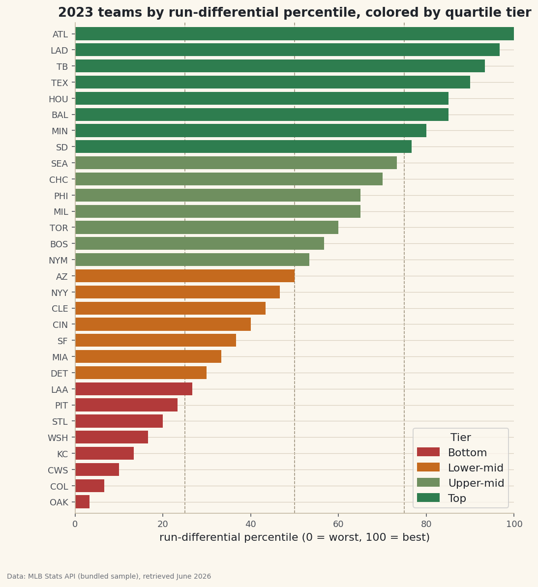
A percentile-ranked bar chart of every team, colored into four quartile tiers.
A raw rank tells you a team is 8th of 30. A percentile rank tells you it's at the 73rd percentile — and here's why that's better: a position from 0 to 1 means the same thing whether the pool is 30 teams or 300 players, so scouting reports and projection systems lean on it instead of raw ranks. To show the idea in action I'll score every 2023 team by run-differential percentile, then chop the field into four quartile tiers.
This builds on Summary Statistics and Distributions. The data is the bundled sample_standings.csv (real 2023 MLB standings), so it runs offline.
-
Percentile rank in one call
rank(pct=True)returns each row's rank as a fraction of the field instead of an integer. Multiply by 100 to read it as a familiar percentile.python import pandas as pd df = pd.read_csv("sample_standings.csv") df["RD_pct"] = df["RunDiff"].rank(pct=True) # 0.0 (worst) to 1.0 (best)The best team lands at 1.0, the worst near 0.03 (1/30), and the median team at roughly 0.5. Unlike a raw rank, this number is comparable across seasons of different sizes or across leagues with different team counts — "90th percentile" is "90th percentile" everywhere.
-
Tiers with qcut()
Where
rankgives a continuous position,qcutchops the column into equal-count buckets. Four buckets give quartile tiers with about the same number of teams in each.python tiers = ["Bottom", "Lower-mid", "Upper-mid", "Top"] df["Tier"] = pd.qcut(df["RunDiff"], 4, labels=tiers) out = df.sort_values("RD_pct", ascending=False)[["Team", "RunDiff", "RD_pct", "Tier"]] out["RD_pct"] = (out["RD_pct"] * 100).round().astype(int) print(out.head(10).to_string()) print(df["Tier"].value_counts().reindex(tiers).to_string())Percentiles and tiers, best to worstTeam RunDiff RD_pct Tier 0 Braves 231 100 Top 2 Dodgers 207 97 Top 3 Rays 195 93 Top 7 Rangers 165 90 Top 5 Astros 129 85 Top 1 Orioles 129 85 Top 10 Twins 119 80 Top 14 Padres 104 77 Top 9 Mariners 99 73 Upper-mid 13 Cubs 96 70 Upper-mid teams per tier: Tier Bottom 8 Lower-mid 7 Upper-mid 7 Top 8
Note
qcutsplits by quantity of teams, not by value: each tier holds roughly a quarter of the league regardless of how lopsided the run-differential gaps are. That's the difference fromcut, which would split the value range into equal-width bands and could leave a tier empty. -
Color the bars by tier
A horizontal bar of each team's percentile, colored by its tier, shows the continuous score and the discrete bands at once. Dashed lines at the 25th, 50th, and 75th percentiles mark where the tiers change hands.
python import matplotlib.pyplot as plt tier_color = {"Bottom": "#B23A3A", "Lower-mid": "#C56A1E", "Upper-mid": "#6F8F5F", "Top": "#2E7D4F"} s = df.sort_values("RD_pct") fig, ax = plt.subplots(figsize=(8, 9)) ax.barh(s["Abbr"], s["RD_pct"] * 100, color=[tier_color[t] for t in s["Tier"]]) for q in (25, 50, 75): ax.axvline(q, color="#9A8F79", lw=0.8, ls="--") ax.set_xlabel("run-differential percentile") fig.savefig("percentile_bars.png", dpi=144, bbox_inches="tight")Data: Bundled sample (2023 MLB standings), retrieved June 2026 Because the bars are sorted, the color bands stack cleanly and the dashed lines fall right where one color gives way to the next — a visual confirmation that the percentile and the tier tell the same story two ways.
Troubleshooting
qcut raises a "Bin edges must be unique" error
Too many tied values share a quantile edge, so two bin boundaries collide. Pass duplicates="drop" to merge them (you'll get fewer tiers than requested), or bin a column with more distinct values.
My tiers have unequal counts
With 30 teams and 4 tiers you can't split evenly — qcut hands the remainder out, so you'll see sizes like 8/7/7/8. That's expected. If you need exactly equal groups, the row count must be divisible by the number of tiers.
Should I use rank(pct=True) or qcut?
Different jobs. rank(pct=True) gives a smooth 0-1 score for sorting or thresholding ("top 10%"). qcut gives labeled groups for grouping or coloring. They pair well: score with one, bucket with the other, as we did here.
Challenge yourself
Switch to pd.cut(df["RunDiff"], 4) — equal-width value bands instead of equal-count tiers — and compare the group sizes to qcut's. Which teams change tier, and why does one approach leave the extreme bands nearly empty? Then build percentile ranks within each league by grouping on League before calling rank(pct=True).
Get the code
Here's the complete, working script for this tutorial. It runs exactly as shown.
Download the finished script (55_percentile_ranks_and_tiers.py)This script imports a small shared helper (and reads any bundled sample data) that live next to it in /downloads/ — grab these into the same folder so it runs as-is: sdt_common.py.