Ridge Regression From Scratch: Taming Collinear Features
Part 2 of 9 in Machine Learning from Scratch · course bundle (code + data)
What you'll build
A ridge estimator built in pure numpy on three collinear MLB predictors where plain OLS is singular and fails outright, plus the coefficient shrinkage path as the penalty grows.
Ordinary least squares carries a failure mode most tutorials never show you. When two predictors carry the same information, the matrix OLS has to invert goes singular — the coefficients are no longer uniquely defined, and the solver either refuses or returns garbage. This isn't a rare edge case; near-collinear features are everywhere in sports data. Ridge regression fixes it with one small change: add a penalty on the size of the coefficients, and the system becomes solvable and stable again. We'll build the closed-form ridge estimator in pure numpy, watch OLS fail where ridge succeeds, and trace how the coefficients shrink as the penalty grows.
This builds on Correlation and Regression (ridge is regression with a leash) and on Z-Scores (we standardize so the penalty is fair to every feature). The numbers come from the bundled sample_standings.csv, a real copy of the 2023 MLB standings, and the whole thing runs offline.
See also Correlation and Simple Linear Regression, DataField.dev.
-
Build a deliberately collinear problem
We'll predict wins from three columns: runs scored, runs allowed, and run differential. The trap is that
RunDiffis exactlyRS - RA— it adds no new information, it's a linear copy of the other two. Standardize the features so the penalty treats them on one scale, and center the target so we can solve for slopes without an intercept.python import numpy as np, pandas as pd df = pd.read_csv("sample_standings.csv") feats = ["RS", "RA", "RunDiff"] # RunDiff = RS - RA, exactly X = df[feats].to_numpy(float) Xs = (X - X.mean(0)) / X.std(0) # standardize each column y = df["W"].to_numpy(float); yc = y - y.mean() XtX, Xty = Xs.T @ Xs, Xs.T @ ycOLS meets a singular matrixFeatures: ['RS', 'RA', 'RunDiff'] Check: RunDiff == RS - RA ? True Rank of X'X: 2 (needs to be 3 to invert) OLS (lambda = 0) FAILED: singular matrix - the collinear column broke it.
The rank of
X'Xis 2 where it needs to be 3, so plain OLS — ridge with a penalty of zero — throws aLinAlgError. The math literally cannot pick coefficients, because infinitely many combinations fit equally well. -
Add the ridge penalty
Ridge minimizes the squared error plus
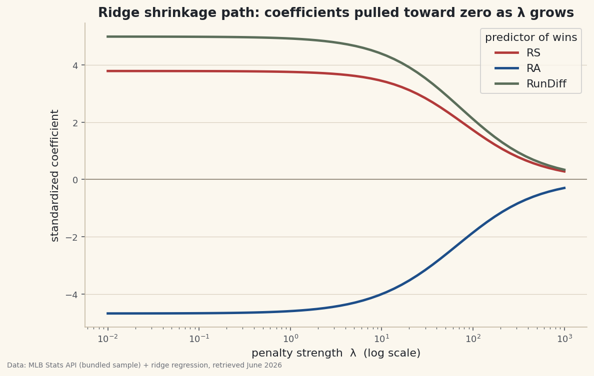
λtimes the squared length of the coefficient vector. That one extra term turns the closed-form solution into(X'X + λI)-1 X'y. Addingλdown the diagonal always makes the matrix invertible — the singular problem becomes solvable for anyλ > 0.python def ridge_fit(lam): n = XtX.shape[0] return np.linalg.solve(XtX + lam * np.eye(n), Xty) for lam in (0.1, 1.0, 10.0, 100.0): print(lam, ridge_fit(lam))Ridge solves, and shrinkslambda= 0.1 RS=+3.788 RA=-4.673 RunDiff=+4.987 |w|=7.81 lambda= 1.0 RS=+3.759 RA=-4.599 RunDiff=+4.927 |w|=7.72 lambda= 10.0 RS=+3.448 RA=-4.005 RunDiff=+4.393 |w|=6.87 lambda= 100.0 RS=+1.726 RA=-1.852 RunDiff=+2.110 |w|=3.30 Ridge always solves - and the coefficients shrink as lambda grows.
At
λ=0.1the coefficient vector has length 7.81; byλ=100it's down to 3.30. The penalty is doing exactly what it promises — pulling the weights toward zero, harder asλrises. -
Trace the shrinkage path
The signature plot of ridge is the coefficient path: each weight against
λon a log scale. Sweepλacross several orders of magnitude and stack the fits.python import matplotlib.pyplot as plt lambdas = np.logspace(-2, 3, 60) paths = np.array([ridge_fit(l) for l in lambdas]) # (60, 3) fig, ax = plt.subplots() for j, name in enumerate(feats): ax.plot(lambdas, paths[:, j], label=name) ax.set_xscale("log"); ax.legend() fig.savefig("ridge_path.png", dpi=144, bbox_inches="tight")Data: Bundled sample (real 2023 MLB standings) + ridge regression, retrieved June 2026 Read it right to left. At small
λthe coefficients sit at their large, unstable values; asλgrows every curve bends toward the zero line. That is the whole idea of regularization in one picture: trade a little bias (coefficients pulled off their least-squares values) for a lot of stability (a solvable, less jumpy model). The same penalty is what keeps models with dozens of overlapping features from overfitting.
Troubleshooting
My OLS didn't error — it returned huge numbers
If your features are nearly collinear rather than exactly collinear, X'X is technically invertible but ill-conditioned, so solve succeeds and hands back wild, sign-flipping coefficients that swing violently on a tiny data change. That instability is the softer version of the same disease, and ridge is the same cure.
How do I choose λ?
Don't eyeball it — pick the λ that minimizes error on data the model didn't train on. That's exactly what k-fold cross-validation is for: score a grid of λ values by cross-validated error and take the best. Ridge without cross-validation is half a method.
Why standardize first?
The penalty is on the raw coefficient sizes, so a feature measured in small units gets an unfairly large coefficient and absorbs more of the penalty. Standardizing puts every feature on a unit-variance scale so λ penalizes them evenhandedly. Note we also don't penalize the intercept — centering the target lets us drop it cleanly.
Challenge yourself
Add a fourth, genuinely informative feature (say, one-run-game record if you have it) and watch its path behave differently from the collinear trio. Then implement the sister method, lasso (an L1 penalty), with coordinate descent and compare the paths — lasso drives coefficients to exactly zero, doing feature selection, while ridge only shrinks them. Finally, wire in cross-validation to pick λ and report the test error at the chosen value versus at λ=0.
Get the code
Want it all in one file? This is the finished script behind this tutorial - the run that produced the outputs above.
Download the finished script (77_ridge_regression_from_scratch.py)This script imports a small shared helper (and reads any bundled sample data) that live next to it in /downloads/ — grab these into the same folder so it runs as-is: sdt_common.py. Or skip the collecting: the Machine Learning from Scratch bundle has this whole course’s scripts and data in one ZIP.