Make a Shot-Density Heatmap with hexbin
What you'll build
Two hexbin maps of 25,000 real NBA shots - a density map of where shots come from and an efficiency map of the make rate by location.
Try to plot 25,000 shots as a scatter and you get a black blob — every interesting pattern buried under overlapping dots. The fix is hexbin: tile the court into hexagons and color each one by what's inside it. It's a histogram in two dimensions, and it's the foundation of every shot chart, heat map, and spatial-density plot you've ever seen. By the end you'll have two maps — where shots come from, and where they actually go in.
This builds on Your First Sports Data Visualization and Binning Data with pd.cut (hexbin is binning in 2D). The data is the bundled nba_league_shots.csv (25,000 real NBA shot locations), so it runs offline.
-
Load the shots and look at the coordinates
Each row is one shot with an
LOC_X(left-right, in feet from center) andLOC_Y(distance up the court). We keep the front-court half, where essentially all shots happen.python import pandas as pd shots = pd.read_csv("nba_league_shots.csv") shots = shots[(shots["LOC_Y"] >= 0) & (shots["LOC_Y"] <= 40)] print(len(shots), "shots") print(shots[["LOC_X", "LOC_Y", "SHOT_MADE"]].head())What's in the fileShots loaded: 24930 X (left-right) range: -25 to 25 feet Y (up the court) range: 1 to 40 feet Overall make rate: 47.3%
Coordinates plus a made/missed flag are all hexbin needs. The hoop sits near
(0, 0); positiveLOC_Ymoves out toward half-court. -
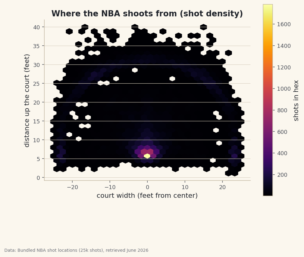
The density map: where shots come from
One call does it.
hexbintakes the x and y arrays, splits the plane into a grid of hexagons (gridsizecontrols how many), and colors each by the count of points inside.mincnt=1hides empty hexes so the court background stays clean.python import matplotlib.pyplot as plt fig, ax = plt.subplots(figsize=(7.5, 7)) hb = ax.hexbin(shots["LOC_X"], shots["LOC_Y"], gridsize=30, cmap="inferno", mincnt=1) fig.colorbar(hb, ax=ax, label="shots in hex") ax.set_aspect("equal") # don't distort the court! fig.savefig("shot_density.png", dpi=144, bbox_inches="tight")Data: Bundled sample (25,000 real NBA shot locations), retrieved June 2026 The shape of the modern NBA appears instantly: a blazing cluster right at the rim, a bright ring along the three-point arc, and a sparse, dim mid-range between them. That
set_aspect("equal")line matters — without it the court stretches and the hexagons turn into ovals, distorting every distance. -
The efficiency map: the real payoff
Density shows where teams shoot; the better question is where they score. hexbin can color each hex by any statistic, not just a count: pass
C=a value per point andreduce_C_function=how to aggregate it. Feed it the made/missed flag withnp.meanand each hex shows its make rate. We require at least 20 shots per hex (mincnt=20) so a lucky 1-for-1 hex doesn't paint a fake 100%.python import numpy as np fig, ax = plt.subplots(figsize=(7.5, 7)) hb = ax.hexbin(shots["LOC_X"], shots["LOC_Y"], C=shots["SHOT_MADE"].astype(float), # the value to aggregate reduce_C_function=np.mean, # mean of made(1)/missed(0) = make rate gridsize=30, cmap="RdYlGn", mincnt=20) fig.colorbar(hb, ax=ax, label="make rate") ax.set_aspect("equal") fig.savefig("shot_efficiency.png", dpi=144, bbox_inches="tight")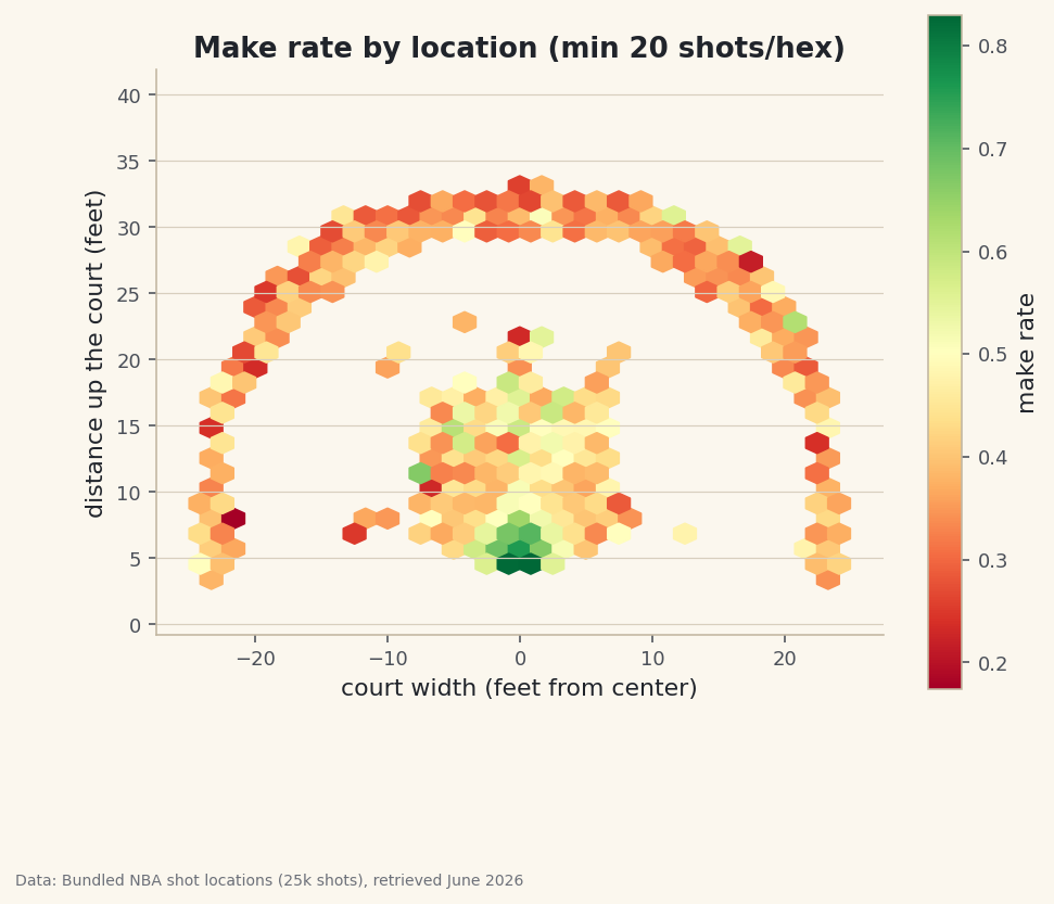
Data: Bundled sample (25,000 real NBA shot locations), retrieved June 2026 That
C/reduce_C_functionpair is the trick worth remembering: swap in any column and any function and the same map shows average shot distance, average shot value, anything per location. It turns a density plot into an analytics tool. -
Read the map in numbers
A chart should always be backed by the figures. Group by the zone label and check the make rates the colors are showing.
python z = (shots.groupby("BASIC_ZONE") .agg(shots=("SHOT_MADE", "size"), make_rate=("SHOT_MADE", "mean")) .sort_values("shots", ascending=False)) print(z)Make rate by zoneShots and make rate by zone: shots make_rate BASIC_ZONE Restricted Area 7379 65.8 Above the Break 3 7238 36.1 In The Paint (Non-RA) 4971 44.2 Mid-Range 2779 40.9 Left Corner 3 1310 38.9 Right Corner 3 1253 38.2 The restricted area is bright green (high make rate); the long mid-range is the cold yellow band the modern NBA has abandoned.The restricted area converts around 66% and the long mid-range around 41% — the exact gap that pushed the league toward layups and threes. The map didn't just look nice; it pointed straight at the most important strategic shift in modern basketball.
Troubleshooting
My court looks stretched / squished
You're missing ax.set_aspect("equal"). Without it matplotlib scales the x and y axes independently to fill the figure, so a round rim looks like an oval and distances lie. Always set equal aspect for spatial data.
The efficiency map has a few wild 0% or 100% hexes
Those are hexes with almost no shots. Raise mincnt (we used 20) so only hexes with a real sample get colored. It's the 2D version of not trusting a batting average over three at-bats.
How do I pick gridsize?
It's the resolution dial: larger gridsize = more, smaller hexes = finer detail but noisier and more empty cells. Smaller = smoother but blurrier. Try 20, 30, and 50 on the same data and pick the one that shows structure without looking grainy.
Challenge yourself
Make an efficiency map for a single star (filter to one PLAYER_NAME from nba_player_shots.csv) and compare it to the league map — where is this player hot or cold relative to average? Then swap reduce_C_function to show average SHOT_DISTANCE per hex, or color by points-per-shot (a three is worth 1.5× a two) to turn the make-rate map into a shot-value map, the metric teams actually optimize.
Get the code
Here's the complete, working script for this tutorial. It runs exactly as shown.
Download the finished script (66_shot_density_heatmap_hexbin.py)This script imports a small shared helper (and reads any bundled sample data) that live next to it in /downloads/ — grab these into the same folder so it runs as-is: sdt_common.py, sdt_nba.py.