Best-of-Seven Math: Why Series Favor Favorites (and by How Much)

Every spring somebody says it: "over seven games, the better team wins." It's half true, and the half matters. A best-of-seven does favor the favorite — but by an amount you can compute exactly, and it's smaller than the folklore implies. A team that wins 55% of single games wins the series just under 61% of the time, which means the better team still goes home early in about two series out of five. This tutorial builds that number from scratch: an exact closed form from counting arguments, a seeded Monte Carlo to verify it, and then real 2023-24 net ratings to put actual teams on the curve.

This builds directly on Monte Carlo Season Simulation — same philosophy, new shape — and borrows its matchup math from Logistic Regression From Scratch. Data is the bundled nba_ratings.csv and nba_home_results.csv, so everything runs offline, and there's no scipy anywhere: math.comb and numpy carry the whole thing.

1. Get the exact answer by counting how a series can end

   A best-of-seven ends the moment one side collects four wins, so the favorite wins in exactly n games (n = 4, 5, 6 or 7) by going 3-and-(n−4) through the first n−1 games and then winning game n. The number of orderings for that start is the binomial coefficient C(n−1, 3) — this is negative-binomial reasoning, even though we never import a stats library — and each such path has probability p⁴(1−p)ⁿ⁻⁴. Sum the four cases and you have the whole formula. As a cross-check, there's a lovely identity: let both teams play all seven games no matter what, and the team that would have clinched still ends up with four-plus wins — so P(≥ 4 wins in 7) must give the same number by a completely different route.

   import math
   import numpy as np
   
   COEF = [math.comb(n - 1, 3) for n in range(4, 8)]      # 1, 4, 10, 20
   
   def series_prob(p):
       """Exact P(first to 4 wins) when each game is an independent p coin flip."""
       p = np.asarray(p, dtype=float)
       q = 1 - p
       return p**4 * (COEF[0] + COEF[1]*q + COEF[2]*q**2 + COEF[3]*q**3)
   
   def series_prob_playout(p):                             # the cross-check identity
       p = np.asarray(p, dtype=float)
       return sum(math.comb(7, k) * p**k * (1 - p)**(7 - k) for k in range(4, 8))

   Output

   ways to clinch in n games, C(n-1,3) for n=4..7: [ 1  4 10 20]
   
   p (one game)   P(win the series)
       0.50             0.5000
       0.55             0.6083
       0.60             0.7102
       0.65             0.8002
       0.70             0.8740
       0.75             0.9294
       0.80             0.9667
   
   max |first-to-four formula - play-all-seven identity| = 3.33e-16

   There are the two headline numbers: 0.55 → 0.6083 and 0.60 → 0.7102. And read the amplification off the table as you go — the format adds about six points of win probability at p = 0.55, eleven at 0.60, and seventeen at 0.70, so the series length helps mid-strong favorites most; near a coin flip or near certainty there's little left to amplify. The identity check landing at 10⁻¹⁶ is floating-point for "identical," which is what a real cross-check should look like.

2. Verify it the honest way: simulate first-to-four

   The closed form assumed the counting was right. Don't take my word for it — play the series. This simulator deals one game at a time to every series that's still alive and stops each one at its fourth win, which is the actual rule, not the play-all-seven shortcut. If the formula and the simulation were built on different logic and still agree, at least one of us is allowed to relax.

   def simulate_series(p, trials, rng):
       """Play `trials` best-of-sevens game by game, each stopping at the 4th win."""
       wins = np.zeros(trials, dtype=np.int64)
       losses = np.zeros(trials, dtype=np.int64)
       length = np.zeros(trials, dtype=np.int64)
       for _ in range(7):
           live = (wins < 4) & (losses < 4)      # series still undecided
           g = rng.random(live.sum()) < p        # one more game for those
           wins[live] += g
           losses[live] += ~g
           length[live] += 1
       return wins == 4, length
   
   rng = np.random.default_rng(2026)             # fixed seed -> same result every run
   mc = []
   for p in (0.50, 0.55, 0.60, 0.65, 0.70, 0.75, 0.80):
       won, length = simulate_series(p, 200_000, rng)
       mc.append(won.mean())

   Output

   200,000 simulated series per p, seed 2026, first-to-four rules
   
   p (one game)    exact    simulated     diff
       0.50        0.5000    0.5003     +0.0003
       0.55        0.6083    0.6076     -0.0007
       0.60        0.7102    0.7113     +0.0011
       0.65        0.8002    0.7994     -0.0007
       0.70        0.8740    0.8744     +0.0004
       0.75        0.9294    0.9292     -0.0003
       0.80        0.9667    0.9675     +0.0008
   
   at p = 0.55, 30.4% of simulated series went the full seven games

   Two hundred thousand series per point and the worst disagreement with the exact formula is about a thousandth — pure Monte Carlo noise. The simulation also hands you something the closed form kept quiet about: at p = 0.55, 30.4% of series go the full seven games. Game sevens aren't a sign the teams were secretly even; they're just what this distribution does nearly a third of the time.

3. Draw the amplification curve

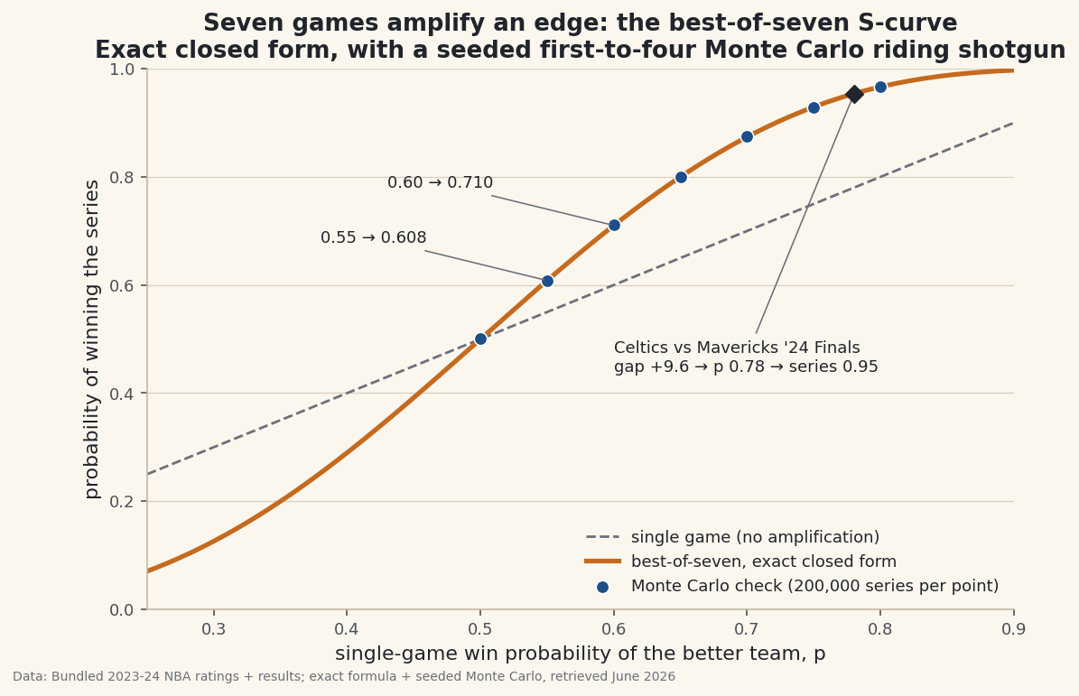
   One chart says all of it: the exact curve, the do-nothing diagonal (a one-game "series" amplifies nothing), and the Monte Carlo estimates sitting on the line they're supposed to sit on. The vertical distance between diagonal and curve is what seven games buy the better team.

   import matplotlib.pyplot as plt
   
   fig, ax = plt.subplots(figsize=(8.6, 5.4))
   pp = np.linspace(0.25, 0.90, 261)
   ax.plot(pp, pp, ls="--", color="#6C7079", label="single game (no amplification)")
   ax.plot(pp, series_prob(pp), lw=2.6, color="#C56A1E", label="best-of-seven, exact")
   ax.scatter([0.50, 0.55, 0.60, 0.65, 0.70, 0.75, 0.80], mc,
              color="#1D4E89", zorder=3, label="Monte Carlo check")
   ax.set_xlabel("single-game win probability of the better team, p")
   ax.set_ylabel("probability of winning the series")
   ax.legend(loc="lower right")
   fig.savefig("series_curve.png", dpi=144, bbox_inches="tight")

   

   The S-shape is the story. Around the middle the curve pulls hard away from the diagonal — small edges compound over seven games — then flattens as certainty approaches, because a huge favorite barely needed the extra games. Flip the reading for underdogs: everything below p = 0.5 gets compressed, which is exactly why a longer series is the last thing an underdog should want.

4. Put real teams on it: net ratings to p, and the 2024 Finals

   The curve needs a p, and this is where an assumption walks in the door — so let's name it. We reuse the exact mapping the logistic-regression tutorial fit on 1,231 real 2023-24 games: P(home win) = sigmoid(w × standardized net-rating gap + b). The intercept b is home advantage, and since we're modeling i.i.d. games on a notional neutral floor, we average each matchup's home and road predictions — by construction, a gap of zero maps to exactly 0.5. Treating a season-long net rating as true strength is a modeling choice, not a fact; it flatters big favorites, and the honest way to use this tool is to remember p is an input you're free to overrule.

   import pandas as pd
   
   ratings = pd.read_csv("nba_ratings.csv")
   nrtg = dict(zip(ratings["Team"], ratings["NRtg"]))
   games = pd.read_csv("nba_home_results.csv")
   games = games[games["home_team"].isin(nrtg) & games["away_team"].isin(nrtg)].copy()
   games["gap"] = games["home_team"].map(nrtg) - games["away_team"].map(nrtg)
   games["home_win"] = (games["home_pts"] > games["away_pts"]).astype(int)
   
   gap_mean, gap_std = games["gap"].mean(), games["gap"].std()
   x = ((games["gap"] - gap_mean) / gap_std).to_numpy()
   y = games["home_win"].to_numpy().astype(float)
   
   def sigmoid(z):
       return 1 / (1 + np.exp(-z))
   
   w, b = 0.0, 0.0
   for _ in range(400):                       # tutorial 71's fit, replayed exactly
       err = sigmoid(w * x + b) - y
       w -= 0.3 * np.mean(err * x)
       b -= 0.3 * np.mean(err)
   
   def game_prob(gap):                        # neutral-floor p: home court averaged away
       p_home = sigmoid(w * (gap - gap_mean) / gap_std + b)
       p_road = 1 - sigmoid(w * (-gap - gap_mean) / gap_std + b)
       return (p_home + p_road) / 2

   Output

   logistic fit on 1,231 real 2023-24 games (identical to tutorial 71):
     w = 1.064, b = 0.217   (b > 0 is home advantage; averaged away below)
   
   net-rating gap   single-game p   best-of-seven
         +2.0           0.565           0.641
         +4.0           0.629           0.763
         +6.0           0.688           0.858
         +9.0           0.766           0.943
        +12.0           0.829           0.981

   Same w and b as tutorial 71 — 1.064 and 0.217 — because it's the same fit on the same games, replayed. The table is the useful artifact: a +2 net-rating edge is a 56.5% game and a 64% series; +6 is a 69% game and an 86% series. Now the worked matchup, end to end:

   gap = nrtg["Boston Celtics"] - nrtg["Dallas Mavericks"]
   p = float(game_prob(gap))
   print(round(gap, 2), round(p, 3), round(float(series_prob(p)), 3))
   
   won, length = simulate_series(p, 200_000, rng)   # same seeded generator
   print(round(won.mean(), 3))

   Output

   Boston Celtics (NRtg +11.71) vs Dallas Mavericks (NRtg +2.09)
   net-rating gap +9.62  ->  single-game p = 0.780
   
   P(Celtics win the series): exact 0.954, simulated 0.954  (200,000 series)
   when they win, how long it takes - in 4: 39.0%, in 5: 34.0%, in 6: 18.7%, in 7: 8.3%

   Boston's historic +11.71 net rating against Dallas's +2.09 gives a +9.62 gap, a 0.780 single game, and a 0.954 series — closed form and simulation agreeing to three decimals. The real 2024 Finals ended Celtics in five, the second-likeliest winning length in our table (34% of Boston's simulated wins take exactly five). One observed series can't validate a probability, of course — but it's satisfying when reality picks an outcome the model considered thoroughly ordinary. The 4.6% Dallas tail was real too; it just didn't come up.

What this model deliberately leaves out

Three simplifications, stated rather than smuggled. First, home-court asymmetry: a real NBA series runs 2-2-1-1-1, the higher seed hosts up to four games, and our fit says home court is worth real percentage points per game — we averaged it away instead of scheduling it, so our p is a neutral-floor compromise. Second, i.i.d. games: we assume the same p every night, independent of the last result — no injuries, no adjustments, no travel, no momentum. Third, net rating as true talent: a season number earned partly against bad teams gets carried into a playoff matchup against a good one. Each of these is fixable with the machinery you just built — the first one is the challenge below — but the fixes move the answer by far less than the jump from folklore to the exact curve did.

Troubleshooting