Bradley-Terry Ratings: Strength From Who You Beat
Part 9 of 9 in NFL Analytics with nflverse · course bundle (code + data)
What you'll build
Bradley-Terry strengths fitted by Hunter's MM algorithm, written by hand with a home-field factor and a one-game prior. On 2025, SEA, DEN and NE all went 14-3 and finish 1st, 3rd and 7th by strength, because their opponents' mean strength was 1.144, 0.704 and 0.627. Without the prior a winless team's first update is exactly zero and an unbeaten team's likelihood keeps rising with no maximum. Out of sample on weeks 13+ of 2010-2025 it ties plain log5 from the record: mean log loss 0.6647 against 0.6651, better in 8 of 16 seasons, a per-game difference whose bootstrap interval straddles zero.
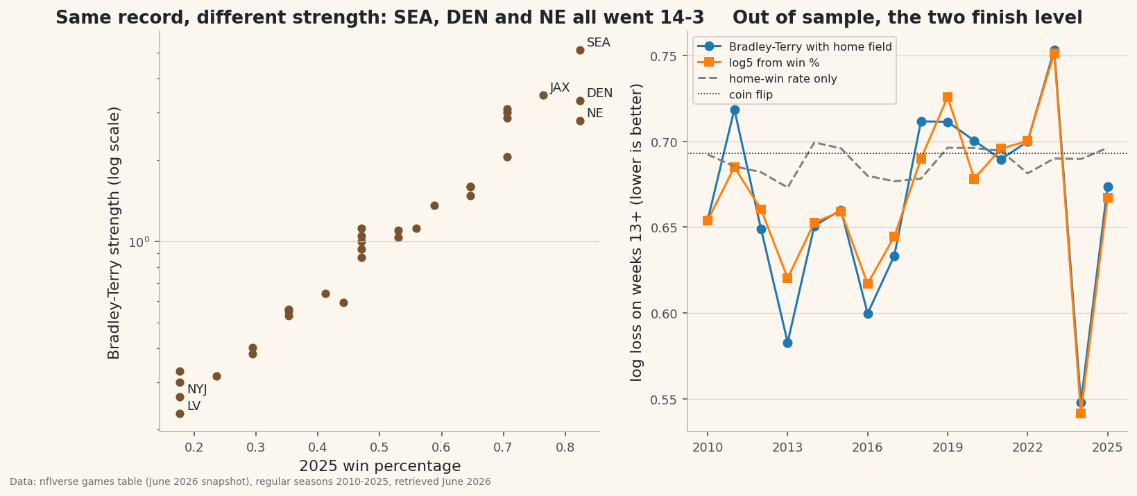
Seattle, Denver and New England all finished the 2025 regular season 14–3. A standings table cannot separate them and a win-percentage model will price them as the same team. They were not the same team, and the reason is in who they beat: Seattle's opponents had a mean strength of 1.144 on the scale this tutorial builds, Denver's 0.704, New England's 0.627. Fit the season with a Bradley–Terry model and the three come out 1st, 3rd and 7th. Then test the model where it matters, on games it has not seen, and it turns out to be exactly as good as the plain win-loss record: a mean log loss of 0.6647 against 0.6651 over sixteen seasons, better in 8 of 16. Both halves of that are worth knowing.
Bring the logistic regression tutorial, because Bradley–Terry is the same model with teams for features, and the Elo tutorial, because Elo is the online, one-game-at-a-time cousin of what is fitted here all at once. Everything runs offline from the bundled nfl_games_lines.csv — every game since 1999 with scores, trimmed from the nflverse games table (June 2026 snapshot). No scipy, no statsmodels, no rating library.
-
The model in one line, and the data
Give every team a positive strength s. Bradley–Terry says team i beats team j with probability si / (si + sj). Double a team's strength and it becomes a 2-to-1 favourite against its old self. Home field enters as a single factor θ multiplying the home side's strength. Fitting means finding the strengths that make the season's actual results most likely. Start with one season, folding the three franchises that changed city, and counting a tie as half a win.
python import pandas as pd import numpy as np FRANCHISE = {"STL": "LA", "SD": "LAC", "OAK": "LV"} # a move is not a new team games = pd.read_csv("nfl_games_lines.csv") games["home_team"] = games.home_team.replace(FRANCHISE) games["away_team"] = games.away_team.replace(FRANCHISE) reg = games[(games.game_type == "REG") & games.home_score.notna()].copy() g25 = reg[reg.season == 2025] print(f"2025: {len(g25)} games, {g25.home_team.nunique()} teams") print(f"home teams won {(g25.home_score > g25.away_score).mean():.4f} of 2025 games")6,967 regular-season games, 272 of them in 2025, one tieregular-season games 1999-2025: 6,967 2025: 272 games, 32 teams, 1 ties home teams won 0.5368 of 2025 games
-
Fit it with the MM algorithm
There is no closed form, but there is a beautifully simple iteration. David Hunter's MM algorithm (2004) updates each team's strength to its wins divided by the sum, over its games, of the weight it had in that game over the game's total strength. Every step is guaranteed to raise the likelihood, so you just repeat it until nothing moves. Strengths are only defined up to a common scale, so each round is normalised to a geometric mean of 1. The prior line is explained in step 4.
python def fit_bt(games, home=True, prior=1.0, iters=5000, tol=1e-12): teams = sorted(set(games.home_team) | set(games.away_team)) ix = {t: i for i, t in enumerate(teams)} h = games.home_team.map(ix).to_numpy() a = games.away_team.map(ix).to_numpy() diff = games.home_score.to_numpy() - games.away_score.to_numpy() hw = np.where(diff > 0, 1.0, np.where(diff < 0, 0.0, 0.5)) wins = np.zeros(len(teams)) np.add.at(wins, h, hw) np.add.at(wins, a, 1 - hw) wins += prior s, theta, home_wins = np.ones(len(teams)), 1.0, hw.sum() for it in range(1, iters + 1): t = theta if home else 1.0 den = t * s[h] + s[a] d = np.zeros(len(teams)) np.add.at(d, h, t / den) np.add.at(d, a, 1 / den) d += 2 * prior / (s + 1.0) new = wins / d new /= np.exp(np.mean(np.log(new))) # strengths are only defined up to scale new_theta = home_wins / np.sum(new[h] / (theta * new[h] + new[a])) if home else 1.0 done = np.max(np.abs(np.log(new / s))) < tol and abs(math.log(new_theta / theta)) < tol s, theta = new, new_theta if done: break return pd.Series(s, index=teams), theta, it166 iterations, theta 1.2262, and three 14-3 teams spread from 1st to 7thconverged in 166 MM iterations home-field factor theta = 1.2262 two equal teams: the home side wins 0.5508 strength wins games win_pct bt_rank pct_rank SEA 5.1261 14.0 17 0.8235 1 1 JAX 3.4831 13.0 17 0.7647 2 4 DEN 3.3118 14.0 17 0.8235 3 1 LA 3.0954 12.0 17 0.7059 4 5 HOU 3.0054 12.0 17 0.7059 5 5 SF 2.8620 12.0 17 0.7059 6 5 NE 2.7930 14.0 17 0.8235 7 1 BUF 2.0520 12.0 17 0.7059 8 5 ... strength wins games win_pct bt_rank pct_rank TEN 0.3001 3.0 17 0.1765 30 29 NYJ 0.2647 3.0 17 0.1765 31 29 LV 0.2301 3.0 17 0.1765 32 29It converges in 166 iterations. The home-field factor comes out at 1.2262, which means two equal teams produce a home win 0.5508 of the time; the raw 2025 home record was 0.5368, and the model's figure is higher because it is measured after accounting for who played whom. The strengths put Seattle top at 5.126 and Las Vegas bottom at 0.230. Read the two rank columns side by side: Jacksonville is 4th by win percentage and 2nd by strength, New England 1st and 7th.
-
Same record, different strength
The whole point of the model is in this comparison. For each of the three 14–3 teams, take the geometric mean strength of the opponents it actually played.
python for team in ("SEA", "DEN", "NE"): mine = g25[(g25.home_team == team) | (g25.away_team == team)] opps = np.where(mine.home_team == team, mine.away_team, mine.home_team) print(team, round(s25[team], 3), round(np.exp(np.mean(np.log(s25[opps]))), 3)) se, ne = s25["SEA"], s25["NE"] print(f"SEA over NE on a neutral field: {se / (se + ne):.4f}")Opponents' mean strength 1.144, 0.704 and 0.627 for the three 14-3 teamsSEA: 14-3, strength 5.126 (rank 1), opponents' mean strength 1.144 DEN: 14-3, strength 3.312 (rank 3), opponents' mean strength 0.704 NE: 14-3, strength 2.793 (rank 7), opponents' mean strength 0.627 SEA over NE on a neutral field: 0.6473
Seattle's schedule was nearly twice as strong as New England's by this measure, 1.144 against 0.627, and the same 14 wins against it are worth nearly twice the strength. On a neutral field the model makes Seattle a 0.6473 favourite over a team with the identical record. This is also the model's blind spot, and it is honest about it: a strength is only as good as the web of games connecting teams, and in one season each team meets fewer than half the league.
-
Why the prior line exists
The textbook model has no answer for a team that has never lost. Four weeks into 2025 two teams were unbeaten and three winless. Run one update with no prior from equal strengths and the winless teams' strength is 0 divided by something — exactly zero — which is a predicted 0% chance of ever winning and a log of zero in the normalisation. The unbeaten side fails more quietly: its likelihood keeps rising as its strength grows, so there is no maximum to find.
python for k in (1, 10, 100, 1000): s_k = s1.copy() s_k["BUF"] = s1["BUF"] * k print(k, round(log_lik(s_k, th1, early), 4))Winless teams hit exactly zero; Buffalo's likelihood keeps climbing as its strength is multiplied upafter 4 weeks: 2 unbeaten ['BUF', 'PHI'], 3 winless ['NO', 'NYJ', 'TEN'] prior 0, first update from equal strengths: NO 0.000, NYJ 0.000, TEN 0.000, BUF 2.000, PHI 2.000 prior 1: converged in 192 iterations, strengths 0.223 to 7.862 BUF's strength x 1: log-likelihood of the 64 real results -26.1431 BUF's strength x 10: log-likelihood of the 64 real results -25.7658 BUF's strength x 100: log-likelihood of the 64 real results -25.7257 BUF's strength x1000: log-likelihood of the 64 real results -25.7217
The fix used throughout is the smallest one that works: every team gets one virtual win and one virtual loss against a reference team of strength 1. It is a prior in the Bayesian sense, it pulls every team slightly toward average, and with 17 real games it barely moves anything. With 4 games it is what keeps the two unbeaten teams finite: the strongest after four weeks, Philadelphia, sits at 7.862 instead of infinity. The log5 comparison in the next step gets exactly the same treatment, one win and one loss added to every record, so the contest is fair.
-
The honest test: games it has not seen
A rating that explains a finished season is easy. For every season from 2010 to 2025, fit on weeks 1–12 and predict every decided game from week 13 on. Compare four forecasts: a coin, the training weeks' home-win rate, log5 from each team's smoothed win percentage (Bill James's head-to-head formula, which uses nothing but the two records), and Bradley–Terry with and without home field. Score with log loss, where lower is better and a coin scores ln 2 = 0.6931.
python for yr in range(2010, 2026): season = reg[reg.season == yr] train, test = season[season.week <= 12], season[season.week > 12] test = test[test.home_score != test.away_score] y = (test.home_score > test.away_score).to_numpy(float) s_h, th, _ = fit_bt(train) p_bt = np.array([p_home(s_h, th, h, a) for h, a in zip(test.home_team, test.away_team)]) rec = team_records(train) wp = (rec.wins + 1) / (rec.games + 2) # the same one-game prior, on the record pa, pb = wp[test.home_team].to_numpy(), wp[test.away_team].to_numpy() p_l5 = (pa - pa * pb) / (pa + pb - 2 * pa * pb) # log5Mean log loss 0.6647 for Bradley-Terry, 0.6651 for log5, and a per-game interval that straddles zeroseason games coin home_rate log5 bt_no_home bt brier_log5 brier_bt 2010 80 0.6931 0.6922 0.6539 0.6522 0.6540 0.2326 0.2287 2011 80 0.6931 0.6854 0.6849 0.7202 0.7186 0.2342 0.2465 2012 80 0.6931 0.6819 0.6603 0.6595 0.6489 0.2315 0.2279 2013 80 0.6931 0.6730 0.6202 0.6073 0.5828 0.2177 0.2023 2014 80 0.6931 0.6993 0.6527 0.6442 0.6507 0.2290 0.2294 2015 80 0.6931 0.6958 0.6590 0.6591 0.6600 0.2314 0.2298 2016 79 0.6931 0.6798 0.6169 0.6228 0.5996 0.2138 0.2071 2017 80 0.6931 0.6767 0.6445 0.6535 0.6333 0.2203 0.2151 2018 80 0.6931 0.6782 0.6898 0.7216 0.7116 0.2469 0.2513 2019 80 0.6931 0.6962 0.7257 0.7088 0.7113 0.2526 0.2459 2020 79 0.6931 0.6961 0.6782 0.6949 0.7003 0.2155 0.2231 2021 92 0.6931 0.6944 0.6957 0.6880 0.6895 0.2386 0.2353 2022 90 0.6931 0.6813 0.7001 0.7160 0.6998 0.2495 0.2468 2023 92 0.6931 0.6900 0.7513 0.7608 0.7533 0.2669 0.2637 2024 93 0.6931 0.6896 0.5415 0.5523 0.5478 0.1802 0.1828 2025 94 0.6931 0.6961 0.6671 0.6632 0.6735 0.2388 0.2413 mean log loss coin 0.6931 home rate 0.6879 log5 0.6651 BT no home 0.6703 BT 0.6647 mean Brier log5 0.2312 BT 0.2298 BT beats log5 in 8 of 16 seasons per game over 1,339 games: log5 minus BT = +0.00033, 95% bootstrap interval -0.01036 to +0.01069
Both real models beat the coin (0.6931) and the home rate (0.6879) comfortably. Against each other they are level. Bradley–Terry averages 0.6647, log5 0.6651; Bradley–Terry wins 8 of 16 seasons; and across all 1,339 test games the per-game difference is +0.00033 with a 95% bootstrap interval from −0.01036 to +0.01069. That interval is more than sixty times wider than the difference. The schedule adjustment is real in-sample and invisible out of sample.
The home-field factor, on the other hand, earns its keep: without it Bradley–Terry scores 0.6703, worse than either. One number for home advantage is worth more to a late-season forecast than thirty-two schedule adjustments. In some seasons both rating models do worse than a coin — 2019 and 2023 among them — because late-season NFL results include teams resting starters and quarterbacks changing, which no rating built from weeks 1–12 can see.
Data: Bundled (nflverse games table, 1999-2026), retrieved June 2026 snapshot (seasons through 2025 complete)
Where this breaks
Five limits. One season is a thin web. Each NFL team plays 17 games against just 14 of the other 31, so a strength leans on chains of results, and a single fluky game between two otherwise unconnected groups can move a whole division. Strength is fixed within the fit. The model treats week 1 and week 17 as the same team; Elo and exponential weighting are the tools for teams that change. Wins only. A 3-point win and a 30-point win count the same, which throws away information a margin-based rating keeps. The prior is a choice. One virtual win and one loss is the smallest stable option, not the best one; a stronger prior would help early in a season and hurt late. The out-of-sample test is one design. Weeks 1–12 predicting 13 and on is a reasonable split, not the only one, and a different split could tip the tie either way.
Sources. Games and scores: the nflverse games table, June 2026 snapshot, bundled by build/make_nfl_lines_csv.py as nfl_games_lines.csv; attribution to nflverse required. Method: the MM algorithm for Bradley–Terry models as set out by David R. Hunter, “MM algorithms for generalized Bradley–Terry models”, The Annals of Statistics 32(1), 2004.
Troubleshooting
My strengths run off to infinity or zero
Some team in your data is unbeaten or winless, and the textbook model has no finite answer for it. Add the prior: one virtual win and one virtual loss against a strength-1 reference team, as in step 4. If you would rather not use a prior, you have to drop that team or wait for it to lose.
My strengths are all multiplied by the same number compared with this page
That is not an error. Bradley–Terry probabilities depend only on ratios of strengths, so any common multiple gives identical predictions. This page normalises to a geometric mean of 1 every iteration; other code may normalise to a sum of 1 or pin one team at 1. Compare ratios, not raw values.
The fit never stops iterating
Check two things. First, the data must be connected: if some group of teams never played anyone outside the group, their strengths relative to everyone else are undetermined. Second, the tolerance: at 1e-12 on log strengths the 2025 fit stops at 166 iterations; a tolerance tighter than floating point can deliver will loop until the iteration cap.
The finished script
Everything this tutorial built, assembled in one runnable file.
Download the finished script (97_bradley_terry_ratings_from_scratch.py)This script imports a small shared helper (and reads any bundled sample data) that live next to it in /downloads/ — grab these into the same folder so it runs as-is: sdt_common.py, sdt_nflverse.py. Or skip the collecting: the NFL Analytics with nflverse bundle has this whole course’s scripts and data in one ZIP.