Quantile Regression: The Whole Margin, Not Just the Average

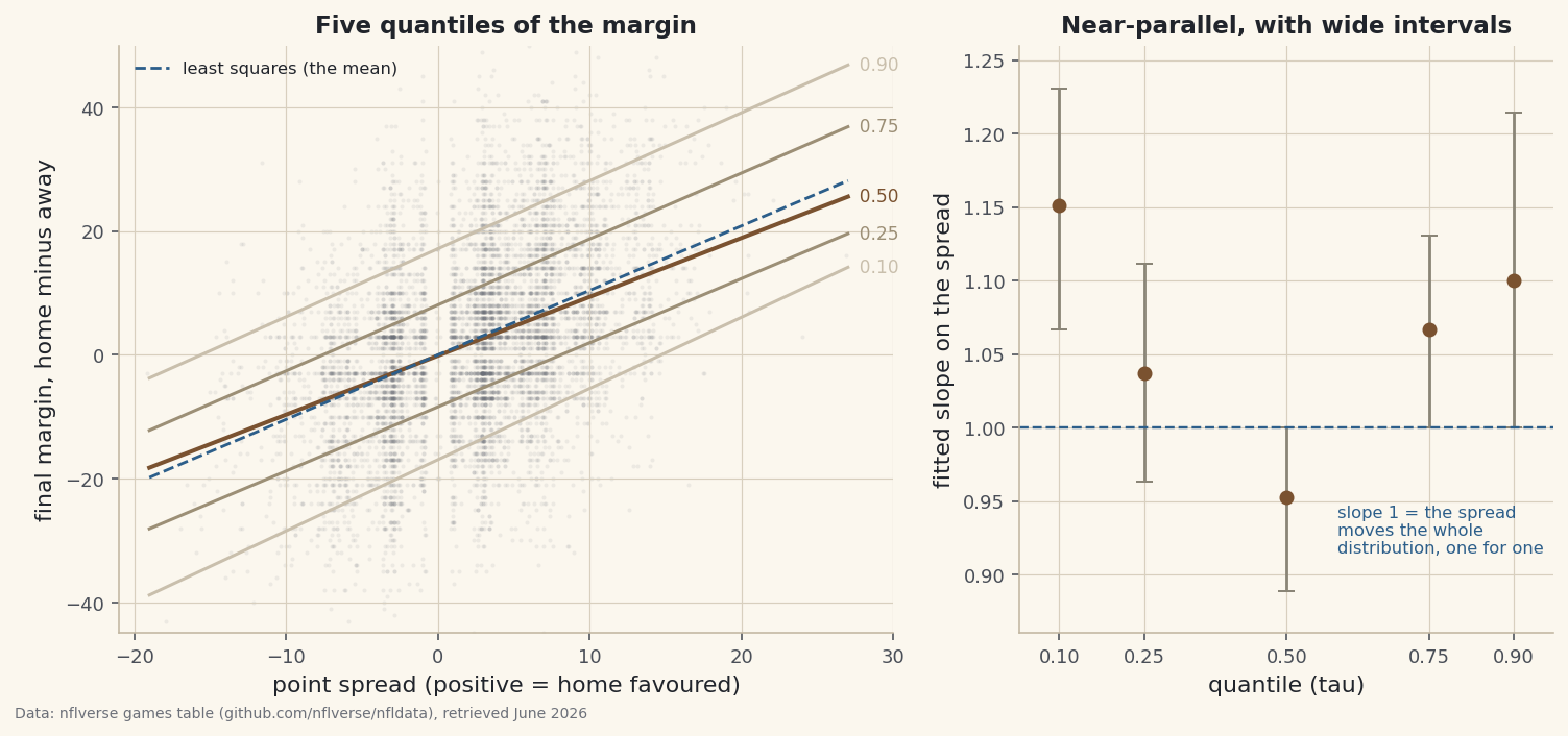
Least squares answers a question nobody asked. Fit the final margin of an NFL game to the point spread across 7,276 games since 1999 and you get margin = −0.0031 + 1.0430 × spread, R-squared 0.1814, residual standard deviation 13.20 points — one line drawn through the middle of a very wide cloud. That line is a conditional mean, and a mean cannot tell you whether a two-touchdown mismatch is a wilder proposition than a coin-flip game, which is the thing anyone pricing a game actually needs to know. Quantile regression fits a line to any percentile you name, so five fits describe the distribution instead of its centre. Written by hand below, the five lines come out near-parallel: the middle 80% of outcomes spans 34.6 points at a 10-point road favourite and 33.4 points at a 14-point home favourite. The spread moves the whole distribution and barely touches its width. It also lands on the median rather than the mean, which is a different claim about what a betting line is.

Bring the regression tutorial, since this is that method with one term changed, and the spread-to-win-probability tutorial, whose one-standard-deviation conversion quietly assumes precisely what this page tests. Everything runs offline from the bundled nfl_games_lines.csv — every game since 1999 with scores and the closing line, trimmed from the nflverse games table (June 2026 snapshot). No scipy, no statsmodels.

1. The mean line, and the question it cannot answer

   Start with what least squares gives you, and keep everything. Ties stay in — all 15 of them — because a tie is a perfectly good margin of zero even though the win-probability tutorial had to drop them. So do the 31 pick’ems and the playoff games. The fit is close to the identity line, which is the market doing its job: a spread of s predicts a margin of about s. The interesting number is the one underneath it. A residual standard deviation of 13.2 points against an R-squared of 0.18 says the spread explains under a fifth of the variation in final margins, and the rest is football.

   import pandas as pd
   import numpy as np
   
   games = pd.read_csv("nfl_games_lines.csv")
   played = games.dropna(subset=["result", "spread_line"])
   x = played.spread_line.to_numpy(float)
   y = played.result.to_numpy(float)
   
   X = np.column_stack([np.ones(len(y)), x])
   a, b = np.linalg.lstsq(X, y, rcond=None)[0]
   resid = y - (a + b * x)
   
   print(len(played), "played games with a line;", int((y == 0).sum()), "ties kept")
   print(f"least squares: margin = {a:+.4f} {b:+.4f} x spread")
   print(f"R-squared {1 - resid.var() / y.var():.4f}, residual sd {resid.std(ddof=2):.4f}")
   print(f"margin overall: mean {y.mean():.4f}, median {np.median(y):.1f}")

   7,276 games, one line, and a residual standard deviation of 13.2 points

   7548 rows in the file, 7276 played games with a line (1999-2025)
     ties kept: 15   pick'ems (spread 0): 31
   
   least squares: margin = -0.0031 +1.0430 x spread
     R-squared 0.1814, residual sd 13.2022 points
   
   margin overall: mean 2.3443, median 3.0
   the mean line is one line. It says nothing about how far from it a game lands.

   Look at the last line of output. The average margin is +2.34 points and the median is +3 — different numbers for the same 7,276 games, because margins pile up on 3 and 7 and then trail off into blowouts, so the mean gets dragged by results the median ignores. Least squares fits the first summary. Nothing in the method lets you ask for the second, or for the 10th percentile.

2. The check loss, and why its minimiser is a quantile

   The trick is to change what you penalise. Squared error punishes misses symmetrically, and its minimiser is the mean. Absolute error punishes them symmetrically but linearly, and its minimiser is the median. Tilt that linear penalty — charge τ per point when you guess too low and 1 − τ when you guess too high — and the minimiser slides to the τ-th quantile. That is the check loss, or the pinball, and the whole method is one line of numpy. To see that it works, take the six wild-card games of the 2025 season and ask for the 75th percentile of their margins by brute force.

   import pandas as pd
   import numpy as np
   import math
   
   def check_loss(r, tau):
       r = np.asarray(r, dtype=float)
       return float(np.sum(np.where(r > 0, tau * r, (tau - 1) * r)))
   
   def quantile_of(v, tau):                       # the minimiser is an order statistic
       s = np.sort(np.asarray(v, dtype=float))
       k = min(max(int(math.ceil(tau * len(s))) - 1, 0), len(s) - 1)
       return float(s[k])
   
   played = pd.read_csv("nfl_games_lines.csv").dropna(subset=["result", "spread_line"])
   wc = played[(played.season == 2025) & (played.game_type == "WC")]
   slate = np.sort(wc.result.to_numpy(float))
   
   print("2025 wild-card margins:", [int(v) for v in slate])
   for c in slate:
       print(f"  a = {c:+6.1f}   check loss at tau=0.75 = {check_loss(slate - c, 0.75):8.2f}")
   print("ceil(0.75 x 6) = 5th order statistic ->", quantile_of(slate, 0.75))

   Six games, six candidates: the loss is smallest at +4, which is the 5th of 6 sorted margins

   the 6 wild-card games of the 2025 season, home margins sorted:
      [-24, -4, -3, -3, 4, 13]
   
   check loss at tau = 0.75 for each candidate:
      a =  -24.0   loss =    95.25
      a =   -4.0   loss =    25.25
      a =   -3.0   loss =    22.75
      a =   -3.0   loss =    22.75
      a =   +4.0   loss =    19.25   <- smallest
      a =  +13.0   loss =    23.75
   
   rule: the minimiser is order statistic ceil(tau*n) = ceil(0.75 x 6) = 5, which is +4
   
   same thing on all 7,276 games - IRLS with only an intercept vs the order statistic:
      tau 0.10   IRLS -16.4803   order statistic  -17.0   loss    18859.1 vs    18858.9
      tau 0.25   IRLS  -7.0000   order statistic   -7.0   loss    32965.3 vs    32965.2
      tau 0.50   IRLS   3.0000   order statistic   +3.0   loss    41083.5 vs    41083.5
      tau 0.75   IRLS  11.0000   order statistic  +11.0   loss    34245.8 vs    34245.8
      tau 0.90   IRLS  21.0000   order statistic  +21.0   loss    19367.9 vs    19367.9

   The six margins are −24, −4, −3, −3, +4 and +13, and the arithmetic at the winner is small enough to check on paper. Guess +4: one game finished above it, by 9, costing 0.75 × 9 = 6.75; four finished below it by 28, 8, 7 and 7, costing 0.25 × 50 = 12.50; total 19.25. Guess −3 instead and the bill is 22.75, because you are now under-predicting two games at the expensive rate. Guess +4.5, which is not a game at all, and it rises to 19.50. The minimum sits exactly on the ceil(0.75 × 6) = 5th sorted value, which is the definition of a sample quantile, and that is the entire justification for the method. The output block then repeats the exercise on all 7,276 margins, where the check loss reproduces the order statistics −17, −7, 3, 11 and 21.

   One honest wrinkle shows up there. At τ = 0.10 the iterative solver of the next step stops at −16.48 rather than −17, for a loss of 18,859.1 against the optimum’s 18,858.9: with thousands of tied integer margins the loss has a flat stretch and the solver stalls inside it. When all you want is a quantile, sort the column.

3. Quantile regression by iteratively reweighted least squares

   Now put a line back in. Minimising the check loss over a slope and an intercept has no closed form, but it has a good trick: |r| = r² / |r|, so absolute error is weighted squared error with weight 1/|r|. Weight each row by τ or 1 − τ over its own residual, solve the weighted normal equations, recompute the residuals, repeat. That is Schlossmacher’s iteration, it is nine lines, and eps exists to stop a point that lands exactly on the line from dividing by zero.

   import pandas as pd
   import numpy as np
   
   def qreg(X, y, tau, iters=500, eps=1e-9):
       b = np.linalg.lstsq(X, y, rcond=None)[0]
       for _ in range(iters):
           r = y - X @ b
           w = np.where(r > 0, tau, 1 - tau) / np.maximum(np.abs(r), eps)
           XW = X * w[:, None]
           nb = np.linalg.solve(X.T @ XW, XW.T @ y)
           if np.max(np.abs(nb - b)) < 1e-12:
               return nb
           b = nb
       return b
   
   played = pd.read_csv("nfl_games_lines.csv").dropna(subset=["result", "spread_line"])
   x = played.spread_line.to_numpy(float)
   y = played.result.to_numpy(float)
   X = np.column_stack([np.ones(len(y)), x])
   
   for tau in (0.10, 0.25, 0.50, 0.75, 0.90):
       a, b = qreg(X, y, tau)
       on_line = int((np.abs(y - (a + b * x)) < 1e-9).sum())
       print(f"tau {tau:.2f}   a = {a:8.4f}   b = {b:7.4f}   games on the line: {on_line}")

   Five fits, each landing on exact fractions, and each running through real games

   quantile regression on 7,276 games:  margin = a + b x spread
   
    tau        a         b     games exactly on the line     R1
    0.10  -16.9394   1.1515            6                0.1077
    0.25   -8.4074   1.0370            6                0.0928
    0.50   -0.1429   0.9524           51                0.0908
    0.75    8.0667   1.0667           14                0.1009
    0.90   17.1500   1.1000            9                0.0943
   
   the median line runs through 51 real games, at just 2 distinct (spread, margin) pairs:
      [(-3.0, -3), (7.5, 7)]
   
   same five fits on the 285 games of 2025 alone, IRLS vs brute force over all 40470 pairs of games:
      tau 0.10   IRLS a= -15.609 b=1.3043   brute a= -15.609 b=1.3043   loss  578.7783 vs  578.7783
      tau 0.25   IRLS a=  -7.767 b=1.1333   brute a=  -7.767 b=1.1333   loss 1091.5583 vs 1091.5583
      tau 0.50   IRLS a=   0.500 b=1.0000   brute a=   0.500 b=1.0000   loss 1377.2500 vs 1377.2500
      tau 0.75   IRLS a=   8.722 b=1.2222   brute a=   8.722 b=1.2222   loss 1100.2639 vs 1100.2639
      tau 0.90   IRLS a=  15.421 b=1.2463   brute a=  15.444 b=1.2444   loss  640.0116 vs  640.0111   <- a vertex short

   Two things in that output are worth more than the coefficients. First, every fitted slope is a tidy fraction — 38/33, 28/27, 20/21, 16/15, 11/10 — and that is not a coincidence. The optimum of a check-loss fit sits at a vertex where the line passes exactly through data points, so its coefficients are ratios of real game numbers. Second, the column counting games on the line confirms it: 6 for the 10th percentile, 51 for the median. Those 51 games sit at only two distinct coordinates — every game where the road team was favoured by 3 and won by exactly 3, which is a push on the number, and every game where the home team was favoured by 7.5 and won by exactly 7, which is a half-point short of one.

   That property is also how you prove the solver right without trusting it. For one season, 285 games and 40,470 pairs, you can simply fit the line through every pair of games and keep the one with the smallest loss. The script does that, and the exact answer and the iteration agree to the digit at four of the five percentiles; at the fifth the iteration stops one vertex short, with a loss larger by less than one part in ten thousand. That is the honest character of this solver — fast, and occasionally a hair off a corner. The last column, Koenker and Machado’s R1, is the check-loss analogue of R-squared: between 0.091 and 0.108, so the spread buys you about a tenth of the way from a flat line to a perfect one at every percentile. This is a weak-signal problem and the method does not disguise it.

4. Read the fan

   Five lines, five slopes, and the slopes are the whole answer. If the spread only moved the distribution up and down, every slope would be 1 and the lines would be parallel. If big favourites were genuinely more volatile, the upper slopes would exceed the lower ones and the fan would open to the right. What the fit gives is the first picture with a wobble: slopes of 1.1515, 1.0370, 0.9524, 1.0667 and 1.1000, none of them further than 0.16 from one, and no two lines crossing anywhere in the observed range of −19 to +27.

   import pandas as pd
   import numpy as np
   
   # fits from the previous block, as exact fractions
   FIT = {0.10: (-559 / 33, 38 / 33), 0.25: (-227 / 27, 28 / 27), 0.50: (-1 / 7, 20 / 21),
          0.75: (121 / 15, 16 / 15), 0.90: (343 / 20, 11 / 10)}
   
   print(" spread     q10     q25     q50     q75     q90   80% band")
   for s in (-10, -3, 0, 3, 7, 14):
       v = [a + b * s for a, b in FIT.values()]
       print(f"  {s:+5.1f}  {v[0]:6.2f}  {v[1]:6.2f}  {v[2]:6.2f}  {v[3]:6.2f}  {v[4]:6.2f}"
             f"     {v[4] - v[0]:6.2f}")
   print("band slope:", round(FIT[0.90][1] - FIT[0.10][1], 4), "points per point of spread")

   The 80% band shrinks by 1.2 points across a 24-point swing in the spread, and the bootstrap says even that is noise

   where the five lines sit, by spread:
   
    spread     q10     q25     q50     q75     q90   80% band
     -10.0  -28.45  -18.78   -9.67   -2.60    6.15      34.60
      -3.0  -20.39  -11.52   -3.00    4.87   13.85      34.24
      +0.0  -16.94   -8.41   -0.14    8.07   17.15      34.09
      +3.0  -13.48   -5.30    2.71   11.27   20.45      33.93
      +7.0   -8.88   -1.15    6.52   15.53   24.85      33.73
     +14.0   -0.82    6.11   13.19   23.00   32.55      33.37
   
   the 80% band changes by -0.0515 points per point of spread: 34.60 wide at a 10-point road favourite, 33.37 at a 14-point home favourite.
   lines crossing anywhere in the observed range (-19 to 27): 0
   
   slopes with a 95% pairs-bootstrap interval (200 resamples):
      tau 0.10   b = 1.1515   [1.0667, 1.2310]   <- clear of 1
      tau 0.25   b = 1.0370   [0.9630, 1.1111]
      tau 0.50   b = 0.9524   [0.8889, 1.0000]
      tau 0.75   b = 1.0667   [1.0000, 1.1304]
      tau 0.90   b = 1.1000   [1.0000, 1.2143]

   The band between the 10th and 90th percentiles measures 34.60 points at a 10-point road favourite and 33.37 at a 14-point home favourite: it narrows by 0.0515 points for every point of spread, which over that whole 24-point swing is 1.2 points out of 34. Set against it, the interquartile band moves the other way, widening by 0.0296 points per point. Two measures of the same alleged effect with opposite signs and trivial magnitudes is what no effect looks like. The pairs bootstrap agrees: 200 resamples put the five slopes in intervals between 0.11 and 0.21 wide, and four of them either contain 1 or stop exactly on it. The exception is the 10th percentile at [1.067, 1.231], and before making anything of it, note it is one of five intervals read at once — the multiple-comparisons tutorial exists for exactly this temptation. The bootstrap itself is the resampling tutorial’s method applied to a statistic with no convenient standard error.

   

5. The same question with no model at all

   A fitted slope is an argument. Before publishing one, ask the file the same question in a way that assumes nothing: subtract the spread from the margin, and group what is left by how big the line was. If the spread is a pure location shift, that residual has the same distribution in every group — no linearity, no estimator, no percentile chosen in advance.

   import pandas as pd
   import numpy as np
   
   played = pd.read_csv("nfl_games_lines.csv").dropna(subset=["result", "spread_line"]).copy()
   played["resid"] = played.result - played.spread_line
   played["band"] = pd.cut(played.spread_line.abs(), [-0.01, 2.5, 6.5, 10.5, 30],
                           labels=["0-2.5", "3-6.5", "7-10.5", "11+"])
   
   for lab, d in played.groupby("band", observed=True):
       p10, p50, p90 = np.percentile(d.resid, [10, 50, 90])
       print(f"|line| {lab:<8} n={len(d):>5}  p10 {p10:6.1f}  p50 {p50:5.1f}  p90 {p90:6.1f}"
             f"   80% band {p90 - p10:5.1f}")
   
   for s in (-7.0, -3.0, -1.0, 1.0, 3.0, 4.0, 6.0, 7.0, 10.0):
       d = played[played.spread_line == s].result
       print(f"spread {s:+5.1f}  n={len(d):>4}  median {d.median():+5.1f}  mean {d.mean():+6.2f}")

   Four buckets, four 80% bands: 34.0, 34.0, 34.0 and 33.5 points

   the same question with no model at all - margin minus spread, by size of line:
   
     |line|      n     p10    p50     p90    width
     0-2.5     1481   -16.5   -0.5    17.5     34.0
     3-6.5     3593   -17.0   -0.5    17.0     34.0
     7-10.5    1648   -16.0    0.0    18.0     34.0
     11+        554   -15.5    0.0    18.0     33.5
   
   where the median lands at every whole-number line posted 150+ times:
   
     spread      n   median   mean    median - spread
      -7.0    158     -7.0   -8.55          exact
      -3.0    498     -3.0   -2.98          exact
      -1.0    261     -2.0   -0.22          -1
      +1.0    285     -1.0   -0.06          -2
      +3.0    655     +3.0   +2.48          exact
      +4.0    227     +5.0   +4.77          +1
      +6.0    237     +5.0   +4.95          -1
      +7.0    333     +7.0   +8.90          exact
     +10.0    166    +10.0  +10.93          exact
   
   5 of 9 land exactly on the line - and they are the key numbers football scores in.

   The four bands come out at 34.0, 34.0, 34.0 and 33.5 points on samples of 1,481, 3,593, 1,648 and 554 games. A pick’em and a two-touchdown mismatch have the same spread of outcomes around their respective lines, to within half a point, and the fitted fan was telling the truth.

   The second table is the one I did not expect. At the five whole-number lines football actually scores in — ±3, ±7 and 10 — the median margin is exactly the spread: −7 on 158 games, −3 on 498, +3 on 655, +7 on 333, +10 on 166. The means at those same lines are not: a 7-point home favourite won by an average of 8.90, and a 7-point road favourite by 8.55. At the four other whole-number lines with comparable samples the median misses by a point or two in both directions, so this is five hits out of nine and I have shown you all nine. But the five hits are not a random five, and the reading is that the market is posting a number it expects the game to land on as often above as below — a median forecast, priced in the currency of percentiles rather than averages.

6. Score it where it was not fitted

   Everything so far was measured on the games that produced it. The discipline from the train/test tutorial applies with a time split: fit the five lines on 1999 through 2019, then count what share of the held-out 2020-2025 games fall below each. A 25th-percentile line doing its job has about a quarter of future games beneath it.

   import pandas as pd
   import numpy as np
   
   def qreg(X, y, tau, iters=500, eps=1e-9):
       b = np.linalg.lstsq(X, y, rcond=None)[0]
       for _ in range(iters):
           r = y - X @ b
           w = np.where(r > 0, tau, 1 - tau) / np.maximum(np.abs(r), eps)
           XW = X * w[:, None]
           nb = np.linalg.solve(X.T @ XW, XW.T @ y)
           if np.max(np.abs(nb - b)) < 1e-12:
               return nb
           b = nb
       return b
   
   played = pd.read_csv("nfl_games_lines.csv").dropna(subset=["result", "spread_line"])
   train, test = played[played.season <= 2019], played[played.season >= 2020]
   Xt = np.column_stack([np.ones(len(train)), train.spread_line.to_numpy(float)])
   xe, ye = test.spread_line.to_numpy(float), test.result.to_numpy(float)
   
   for tau in (0.10, 0.25, 0.50, 0.75, 0.90):
       a, b = qreg(Xt, train.result.to_numpy(float), tau)
       print(f"tau {tau:.2f}   fitted on {len(train)} games   "
             f"share of the {len(ye)} held-out games below it: {(ye < a + b * xe).mean():.4f}")

   Fitted on 5,583 games, scored on 1,693: every nominal level within 2.2 points

   fit on 5583 games (1999-2019), scored on 1693 games (2020-2025):
   
     tau   fitted line                share of held-out games below it
     0.10   margin = -17.5000 +1.1667 x spread        0.0780
     0.25   margin =  -8.6400 +1.0400 x spread        0.2310
     0.50   margin =  -0.1429 +0.9524 x spread        0.4903
     0.75   margin =  +8.1053 +1.0526 x spread        0.7513
     0.90   margin = +17.2727 +1.0909 x spread        0.9067
   
     inside the 80% band: 0.8287   inside the 50% band: 0.5204
     worst miss on a nominal level: 0.0220
   
     sd of (margin - spread): 13.3640 in 1999-2019, 12.6625 in 2020-2025

   The five lines come back at 7.80%, 23.10%, 49.03%, 75.13% and 90.67% against nominal levels of 10, 25, 50, 75 and 90 — a worst miss of 2.2 points, and 82.87% of held-out games inside the 80% band rather than 80%. The misses are not random, though. Both tails are pulled in: fewer extreme games below the bottom line and fewer above the top one, exactly the signature of a slightly narrower distribution. The last line of output confirms it directly: the standard deviation of margin minus spread falls from 13.36 points in 1999-2019 to 12.66 in 2020-2025. The modern game is a little more predictable than the one the lines were fitted on, which is the same drift the win-probability tutorial found from the other direction, and it is the reason a band fitted on 1999 data over-covers today.

Where this breaks

Six limits. Ties and key numbers make the quantiles lumpy. Margins are whole points that pile up on 3 and 7, so a sample quantile is an order statistic that jumps rather than glides, and a half-point move in the data can shift a fitted slope from 16/15 to something else. The solver is not exact. The iteration stalls where the loss goes flat, which cost it half a point at the 10th percentile with no slope to fit; the brute-force check exists because of that, and it only scales to one predictor and a few hundred rows. There are no standard errors in the fit. I bootstrapped the slopes because the analytic variance of a quantile regression depends on the density of the residuals at the line, which is awkward to estimate; Koenker’s rank-inversion intervals are the principled alternative. Fitted quantile lines can cross. These five do not, anywhere between a 19-point road favourite and a 27-point home favourite, but nothing in the method prevents it and extrapolating past the observed range invites it. Each line is straight because I made it straight. Curvature in a tail would show up as a bad fit, not as a warning. And conditioning on the spread is conditioning on a market. These are the games as the closing line saw them; the spread already contains the injuries, the weather and the public, so none of this measures how predictable football is — only how predictable it is once a betting market has spoken.

Sources. Games, scores and closing lines: the nflverse games table (public; attribution to nflverse required), June 2026 snapshot, bundled as nfl_games_lines.csv. The method: Roger Koenker and Gilbert Bassett Jr., “Regression Quantiles,” Econometrica 46(1), 1978, pp. 33-50, doi:10.2307/1913643. The goodness-of-fit measure: Roger Koenker and José A. F. Machado, “Goodness of Fit and Related Inference Processes for Quantile Regression,” Journal of the American Statistical Association 94(448), 1999, pp. 1296-1310, doi:10.1080/01621459.1999.10473882. The iteration: E. J. Schlossmacher, “An Iterative Technique for Absolute Deviations Curve Fitting,” Journal of the American Statistical Association 68(344), 1973, pp. 857-859, doi:10.1080/01621459.1973.10481436. Every number on this page is recomputed by the tutorial’s script, whose asserts fail rather than print a figure they cannot reproduce.

Troubleshooting