Point Spread to Win Probability: Calibrate the Line on 7,261 NFL Games

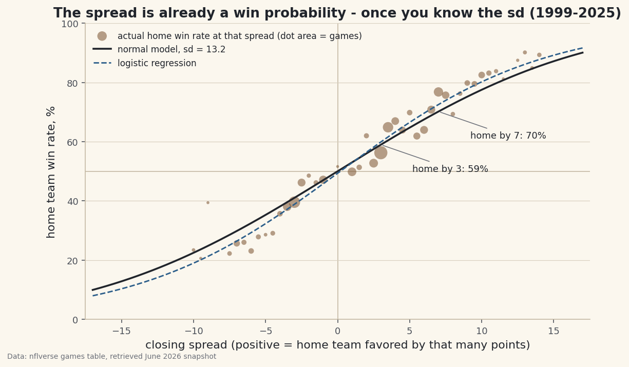
A point spread answers one question — by how much? — and the question people actually ask is a different one: how often? Those two are linked by a single number, and this tutorial estimates it. Across 7,261 decided NFL games with a closing line, from the 1999 season through 2025, the final margin lands within a standard deviation of 13.2 points of the spread. That one number turns any spread into a win probability: a 3-point favorite is a 59.0% proposition, a 7-point favorite 70.2%, a 14-point favorite 85.5%. Then the file talks back. Real 3-point favorites won 58.1% of 1,152 games, right on the curve; real 7-point favorites won 76.0%, six points above it — while covering only 47.3% of the time. Winning and covering are different questions, and the last section prices the opening week of 2026 to show why that matters.

You need pd.cut for the bins and it helps to have built a logistic regression by hand, because we fit one here in nine lines. Everything runs offline from the bundled nfl_games_lines.csv — every game since 1999 with scores and the closing spread, trimmed from the nflverse games table. The 2026 schedule is in the file too, with blank scores, which is the first thing you have to handle.

1. Load it, filter it, and learn which way the sign points

   The file has 7,548 rows but only 7,276 have been played, and 15 of those ended tied — a tie is neither a home win nor a home loss, so for a win-probability model it is dropped, and said so. That leaves 7,261 decided games with a closing line. The column you must not guess about is spread_line: nflverse stores it from the home team’s side, positive when the home team is favored. Do not take the documentation’s word for it — correlate the spread with result (home score minus away score). The sign of that correlation is the sign convention, and +0.426 settles it.

   import pandas as pd
   import numpy as np
   
   games = pd.read_csv("nfl_games_lines.csv")
   played = games.dropna(subset=["result", "spread_line"])
   dec = played[played.result != 0].copy()          # ties are neither outcome
   dec["home_win"] = (dec.result > 0).astype(int)
   
   print(len(games), "rows,", len(played), "played,", len(dec), "decided with a line")
   print("corr(spread, result) =", round(np.corrcoef(dec.spread_line, dec.result)[0, 1], 3))
   print("home win rate:", round(100 * dec.home_win.mean(), 1), "%")

   7,261 decided games; the sign convention read off the data, not the docs

   7548 rows in the file, seasons 1999-2026
   7276 played, 7353 carry a spread, 7276 both
   15 ties dropped -> 7261 decided games with a closing line
   
              game_id away_team home_team  result  spread_line
   0  1999_01_ARI_PHI       ARI       PHI      -1         -3.0
   1  1999_01_BAL_STL       BAL       STL      17          0.0
   2  1999_01_BUF_IND       BUF       IND      17         -3.0
   
   corr(spread_line, result) = +0.426  -> positive spread = home team favored
   home teams won 56.4% and were favored in 65.0% of games (31 pick'ems)

   Two baselines to carry forward. Home teams won 56.4% of these games — the football entry in the five-league comparison — and the market made them the favorite in 65.0% of them. Any conversion we build has to reproduce the first number from the second, or it is wrong before it starts.

2. The empirical answer: fold to the favorite and bin

   Before any model, ask the file directly. Fold every game to the favorite’s side — the favorite wins when the margin has the same sign as the spread — and bin by the size of the spread. The bin edges are not arbitrary: 3 and 7 get their own bins because those are the margins football produces most often, so the market posts them constantly and a half-point either side changes the price. A second column asks whether the favorite covered: won by more than the spread.

   import pandas as pd
   import numpy as np
   
   dec = pd.read_csv("nfl_games_lines.csv").dropna(subset=["result", "spread_line"])
   dec = dec[dec.result != 0]
   fav = dec[dec.spread_line != 0].copy()                  # drop the 31 pick'ems
   fav["fav_spread"] = fav.spread_line.abs()
   fav["fav_margin"] = fav.result * np.sign(fav.spread_line)
   fav["fav_win"] = (fav.fav_margin > 0).astype(int)
   fav["covered"] = (fav.fav_margin > fav.fav_spread).astype(int)
   
   edges = [0, 2.5, 3, 3.5, 6.5, 7, 7.5, 9.5, 13.5, 30]
   labels = ["0.5-2.5", "3", "3.5", "4-6.5", "7", "7.5", "8-9.5", "10-13.5", "14+"]
   fav["bucket"] = pd.cut(fav.fav_spread, bins=edges, labels=labels)
   table = fav.groupby("bucket", observed=True).agg(
       games=("fav_win", "size"), win_pct=("fav_win", "mean"), cover_pct=("covered", "mean"))
   print((table * [1, 100, 100]).round(1))

   Favorites by spread size: win rate climbs from 52.9% to 91.2%; cover rate never leaves the forties

   7230 decided games with a favorite
   
   favorite's win rate, and cover rate, by size of the spread:
            games  fav_win_pct  covered_pct
   bucket                                  
   0.5-2.5   1446         52.9         49.5
   3         1152         58.1         43.3
   3.5        681         63.7         49.9
   4-6.5     1755         67.9         48.2
   7          488         76.0         47.3
   7.5        291         76.3         47.8
   8-9.5      515         75.9         47.2
   10-13.5    687         83.0         47.0
   14+        215         91.2         45.6
   
   all favorites: won 66.5%, covered 47.5%
   pushes at exactly 3: 9.0% of 1152 games (counted as not covered)
   cover rate at 3 among the 91.0% of games that were decided: 47.6%

   Read the two columns against each other. The win rate does exactly what a spread should make it do: 52.9% for favorites of a field goal or less, 58.1% at exactly 3, 67.9% in the 4-to-6.5 band, 76.0% at exactly 7, 83.0% from 10 to 13.5, and 91.2% for two-touchdown favorites. The cover rate does nothing at all — every bucket sits between 43.3% and 49.9%, and favorites as a group won 66.5% of their games while covering 47.5%. That flat second column is what an efficient line looks like: the spread already contains the favorite’s strength, so beating it is a coin flip no matter how strong the favorite is. Winning is a function of the spread; covering, by construction, is not.

3. The normal model: one number does all the work

   Bins are honest but lumpy — 291 games at 7.5 is a bucket with a ±5-point margin of error — and they say nothing about a 4.5-point favorite at a neutral site. The classic fix, proposed by Hal Stern in 1991, is a model with a single parameter: treat the final margin as the spread plus noise, and let the noise be normal with standard deviation σ. Then the probability the favorite wins is the probability the noise does not overwhelm the spread, Φ(spread / σ). Estimating σ is one line: the standard deviation of result - spread_line. Its mean is the market’s bias, and +0.10 points is as close to zero as a bias gets.

   import pandas as pd
   from math import erf, sqrt
   
   dec = pd.read_csv("nfl_games_lines.csv").dropna(subset=["result", "spread_line"])
   dec = dec[dec.result != 0]
   resid = dec.result - dec.spread_line
   sigma = resid.std()
   print("mean", round(resid.mean(), 2), " sd", round(sigma, 2))
   
   def p_win(spread, s=sigma):                 # standard normal CDF, no scipy needed
       return 0.5 * (1 + erf(spread / s / sqrt(2)))
   
   for s in [1, 3, 7, 10, 14]:
       print(f"{s:>3}-point favorite: {100 * p_win(s):.1f}%")

   sd 13.21 points; the whole lookup table falls out of one Phi() call

   margin minus spread: mean +0.10, sd 13.21 points over 7261 games
   (a mean near zero is the market being unbiased; the sd is the whole model)
   
   P(favorite wins) = Phi(spread / sd):
        1 -point favorite   53.0%
      2.5 -point favorite   57.5%
        3 -point favorite   59.0%
        4 -point favorite   61.9%
      6.5 -point favorite   68.9%
        7 -point favorite   70.2%
       10 -point favorite   77.5%
       14 -point favorite   85.5%
   
   sd by era: 1999-2012 13.53, 2013-2025 12.88

   The standard deviation is 13.21 points, and with it the table writes itself: 53.0% for a 1-point favorite, 59.0% at 3, 70.2% at 7, 77.5% at 10, 85.5% at 14. Compare that to the bins. At 3 the model says 59.0 and the file says 58.1 — agreement. At 7 the model says 70.2 and the file says 76.0. At 14+ the model says roughly 88.7 at the bucket’s typical spread and the file says 91.2. The one-parameter curve is a touch flat: it undersells favorites above a field goal and slightly oversells the smallest ones (54.5 predicted, 52.9 observed). One more number worth a glance before moving on: split by era, σ was 13.53 through 2012 and 12.88 since. The market has got tighter, or the game has; the file cannot say which.

4. Fit the sign directly: logistic regression by Newton’s method

   The normal model predicts the sign of the margin by way of the whole margin. A logistic regression skips the middle step and fits the sign itself: logit P(home win) = a + b × spread. With one feature and 7,261 rows, Newton’s method converges in five iterations, and the code is short enough to read whole — gradient, Hessian, one linear solve per step.

   import pandas as pd
   import numpy as np
   
   dec = pd.read_csv("nfl_games_lines.csv").dropna(subset=["result", "spread_line"])
   dec = dec[dec.result != 0]
   X = np.column_stack([np.ones(len(dec)), dec.spread_line.to_numpy(float)])
   y = (dec.result > 0).to_numpy(float)
   
   beta = np.zeros(2)
   for _ in range(25):
       p = 1 / (1 + np.exp(-X @ beta))
       step = np.linalg.solve(X.T @ (X * (p * (1 - p))[:, None]), X.T @ (y - p))
       beta += step
       if np.abs(step).max() < 1e-10:
           break
   a, b = beta
   print(f"logit = {a:+.4f} + {b:.4f} x spread;  odds x{np.exp(b):.3f} per point")
   for s in [3, 7, 14]:
       print(f"{s:>3}-point favorite: {100 / (1 + np.exp(-(a + b * s))):.1f}%")

   Three columns side by side: the file, the normal curve, the logistic curve

   logit P(home win) = -0.0265 + 0.1426 x spread   (Newton, 5 iterations)
   a pick'em at home: 49.3%   one point of spread multiplies the odds by 1.153
   
   favorite by   empirical (n)     normal   logistic
      0.5-2.5      52.9% (1446)     54.5%     54.7%
            3      58.1% (1152)     59.0%     59.9%
          3.5      63.7% ( 681)     60.4%     61.6%
        4-6.5      67.9% (1755)     64.7%     66.5%
            7      76.0% ( 488)     70.2%     72.5%
      10-13.5      83.0% ( 687)     79.7%     82.4%
          14+      91.2% ( 215)     88.7%     90.5%
   (the normal and logistic columns are evaluated at a typical spread in the bucket)

   The fit is −0.0265 + 0.1426 × spread: a pick’em at home is 49.3% (the intercept is the market’s home-field pricing being almost exactly right), and every point of spread multiplies the favorite’s odds by 1.153. Laid against the bins, the logistic curve is the steeper of the two — 72.5% at 7 against the normal model’s 70.2, 82.4% in the 10-to-13.5 band against 79.7 — and the file sides with it in every bucket above a field goal. The difference is small in absolute terms, two to three points, and it has a plain cause: the normal model is forced to describe blowout margins and one-score margins with the same σ, and the sign of a game does not care how large the blowout was. When the question is the sign, fit the sign.

   

5. Score it where it was not fitted

   A curve that matches the bins it was fitted on has proven little. So fit both models on 1999 through 2019 — 5,573 games — and score them on the 1,688 games of 2020 through 2025 with the Brier score, the mean squared gap between the probability and the outcome. The baseline to beat is the laziest possible forecast: every home team gets the training home-win rate, 57.2%.

   import pandas as pd
   import numpy as np
   from math import erf, sqrt
   
   dec = pd.read_csv("nfl_games_lines.csv").dropna(subset=["result", "spread_line"])
   dec = dec[dec.result != 0]
   train, test = dec[dec.season <= 2019], dec[dec.season >= 2020]
   sigma = (train.result - train.spread_line).std()
   y = (test.result > 0).to_numpy(float)
   
   phi = np.vectorize(lambda z: 0.5 * (1 + erf(z / sqrt(2))))
   p_normal = phi(test.spread_line / sigma)
   p_base = np.full(len(test), (train.result > 0).mean())
   for name, p in [("base rate", p_base), ("normal model", p_normal)]:
       print(f"{name:<14} Brier {np.mean((p - y) ** 2):.4f}")

   Out of sample: the normal model cuts the base rate's Brier score by 15.6%

   fit on 1999-2019 (5573 games), scored on 2020-2025 (1688 games)
   training sd 13.37; training home-win rate 57.2%
   
   model                    Brier  log loss
   always the base rate    0.2495    0.6923
   normal model            0.2106    0.6088
   logistic                0.2099    0.6067
   
   normal model beats the base rate by 15.6% of Brier score
   picking the favorite was right 66.6% of the time in the hold-out

   The base rate scores 0.2495, the normal model 0.2106, the logistic 0.2099 — a 15.6% improvement over knowing nothing, and the two models within a thousandth of each other, which is the honest size of the logistic’s edge once it is not allowed to see the answers. Picking the favorite was right 66.6% of the time on the held-out seasons, which is the same two-in-three that favorites managed across the whole file. If you have done the train/test tutorial, this is the same discipline with a time split instead of a random one: the future never leaks into the fit.

6. Price the opening week of 2026, then check the market’s other number

   The 2026 rows have no scores yet but they do have lines, as bundled in the June 2026 snapshot of the file — opening numbers, not the ones that will close. Run the normal model over week 1 and you have a probability for every game. And the market posts a second instrument that is already a probability in disguise: the moneyline. Convert both sides of each game’s moneyline to implied probabilities, note that they sum to more than one (that surplus is the bookmaker’s margin, the overround), rescale so they sum to one, and you have the market’s own win probability to compare against yours.

   import pandas as pd
   import numpy as np
   from math import erf, sqrt
   
   games = pd.read_csv("nfl_games_lines.csv")
   dec = games.dropna(subset=["result", "spread_line"]); dec = dec[dec.result != 0]
   sigma = (dec.result - dec.spread_line).std()
   phi = np.vectorize(lambda z: 0.5 * (1 + erf(z / sqrt(2))))
   
   w1 = games[(games.season == 2026) & (games.week == 1)].copy()
   w1["p_spread"] = 100 * phi(w1.spread_line / sigma)
   implied = lambda ml: np.where(ml < 0, -ml / (-ml + 100), 100 / (ml + 100))
   h, a = implied(w1.home_moneyline), implied(w1.away_moneyline)
   w1["overround"] = 100 * (h + a - 1)
   w1["p_ml"] = 100 * h / (h + a)                 # the vig removed
   print(w1[["away_team", "home_team", "spread_line", "p_spread", "p_ml"]].round(1).to_string(index=False))
   print("overround:", round(w1.overround.mean(), 1), "%")

   Sixteen games priced two ways; the two market instruments agree to within a few points

   2026 week 1: 16 games, lines as bundled in the June 2026 nflverse snapshot
   
         date away home   venue  spread  p(home) spread  home ML  p(home) ML  gap
   2026-09-09   NE  SEA    Home     3.5            60.4   -205.0        64.5 -4.0
   2026-09-10   SF   LA Neutral     3.0            59.0   -175.0        60.9 -1.9
   2026-09-13  ARI  LAC    Home    11.5            80.8   -625.0        82.7 -1.9
   2026-09-13  ATL  PIT    Home     3.0            59.0   -175.0        60.9 -1.9
   2026-09-13  BAL  IND    Home    -3.5            39.6    160.0        36.9  2.6
   2026-09-13  BUF  HOU    Home    -1.5            45.5   -108.0        49.6 -4.1
   2026-09-13  CHI  CAR    Home    -2.5            42.5    114.0        44.9 -2.4
   2026-09-13  CLE  JAX    Home     7.5            71.5   -340.0        74.1 -2.6
   2026-09-13  DAL  NYG    Home    -1.5            45.5    110.0        45.7 -0.2
   2026-09-13   GB  MIN    Home    -1.5            45.5    105.0        46.8 -1.3
   2026-09-13  MIA   LV    Home     3.0            59.0   -175.0        60.9 -1.9
   2026-09-13   NO  DET    Home     7.0            70.2   -325.0        73.4 -3.2
   2026-09-13  NYJ  TEN    Home     3.0            59.0   -170.0        60.4 -1.4
   2026-09-13   TB  CIN    Home     3.5            60.4   -192.0        63.1 -2.6
   2026-09-13  WAS  PHI    Home     5.5            66.1   -230.0        66.9 -0.8
   2026-09-14  DEN   KC    Home     2.5            57.5   -155.0        58.3 -0.8
   
   bookmaker overround on the moneylines: 4.3% average
   spread-model vs vig-free moneyline: mean gap -1.8 pts, largest 4.1 pts
   the steeper logistic curve instead: mean gap -1.3 pts, largest 5.5 pts
   biggest favorite: LAC by 11.5 over ARI -> 80.8% by the spread, 82.7% by the moneyline

   The overround averages 4.3% — the price of the bet, invisible until you add the two sides. With it removed, the spread-derived probability and the moneyline-derived one land within 4.1 points on every game and average a gap of −1.8: the moneyline consistently likes the favorite a little more than the normal curve does, which is the same flatness the bins exposed in step 3, now visible in the market’s own pricing. The steeper logistic curve narrows the average gap to −1.3. Two games are worth naming. The season opener, New England at Seattle on Wednesday September 9, is Seattle by 3.5 — 60.4% by the spread, 64.5% by the moneyline, the week’s widest disagreement. And the biggest favorite of the week, the Chargers by 11.5 over Arizona, is 80.8% by the spread and 82.7% by the moneyline, the two instruments in near-agreement about a four-in-five game.

What this conversion can and cannot claim

Four limits, plainly. First, the probability belongs to the line, not to the teams. The curve says what happened historically to favorites of a given size; it has no idea why this particular favorite is favored, and every point of team knowledge it contains came from the market that set the number. Second, the 2026 lines are opening lines from a June snapshot; closing lines move, and every historical number here was computed on closing lines, so the week-1 table is a demonstration of the method, not a forecast to hold anyone to. Third, the bins carry sampling error you can read straight off the counts — 215 games in the 14+ bucket is a ±4-point estimate — and the 76.0% at exactly 7 is a real 6-point excess over the normal curve on 488 games, which is close to three standard errors and therefore not something to explain away, but also not something one bucket should be asked to explain. Fourth, neither model sees anything but the spread: the total, the venue, rest and weather are all in the file and all unused. The natural next step is the one the Elo tutorial invites from the other direction — build your own rating, convert it to a probability the same way, and measure it against this curve with the same Brier score.

Sources. Games, scores and closing lines: the nflverse games table (public; attribution to nflverse required), trimmed to the bundled CSV by the site’s build script. The normal-margin model: Hal S. Stern, “On the Probability of Winning a Football Game,” The American Statistician 45(3), 1991, doi:10.1080/00031305.1991.10475798, which proposed exactly this model and estimated the same quantity on 1980s seasons; the 13.21 here is estimated fresh from the file and is not taken from the paper.

Troubleshooting