Survival Curves: How Long NFL Head Coaches Really Last

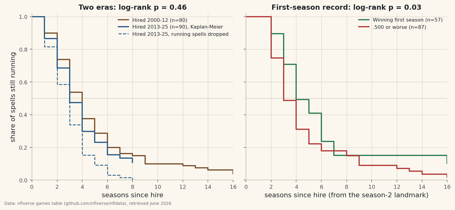
Ask how long an NFL head coach lasts and the obvious method gives the wrong number with complete confidence. Average the finished tenures of every coach hired to open a season since 2000 and you get 4.17 seasons. Split the hires at 2013 and the same arithmetic says recent coaches last 3.03 seasons against 5.10, a leash 40.6% shorter. That gap is mostly an artefact. All 25 spells still running belong to the recent group, including Andy Reid’s 13 seasons in Kansas City and three 2017 hires still in charge after nine. A duration you have not finished watching is right-censored, and survival analysis exists for exactly that. Written by hand below, the Kaplan-Meier estimator puts the median tenure at four seasons, and the log-rank test cannot separate the eras (p = 0.46). It does find one real split, the first-season record, once the clock starts in the right place.

You want the ECDF tutorial first, since a survival curve is one minus an ECDF corrected for unfinished rows, and the chi-square tutorial, since the log-rank statistic is a chi-square with one degree of freedom. Everything runs offline from the bundled nfl_games_coaches.csv: every game from 1999 through the 2026 schedule with each side’s head coach, trimmed from the nflverse games table (June 2026 snapshot). No scipy, no lifelines.

1. Turn games into coaching spells

   No file has a tenure column, so you build one. Stack home and away into one row per team per game, fold the three relocations into their franchises, sort by date, and start a new spell whenever the coach’s name changes. That gives 253 runs, and one of them is wrong. The source credits New Orleans’ 2012 games to Aaron Kromer and Joe Vitt, the season Sean Payton was suspended, so a plain run-length count splits his tenure and invents a one-season hire. My rule is that a coach back with the same team within a season never left. It fires exactly once.

   import pandas as pd
   import numpy as np
   
   games = pd.read_csv("nfl_games_coaches.csv")
   FRANCHISE = {"STL": "LA", "SD": "LAC", "OAK": "LV"}
   
   sides = []
   for me, opp in (("home", "away"), ("away", "home")):
       s = games[["game_id", "season", "game_type", "gameday",
                  f"{me}_team", f"{me}_coach", f"{me}_score", f"{opp}_score"]].copy()
       s.columns = ["game_id", "season", "game_type", "gameday", "team", "coach", "pts", "opp_pts"]
       sides.append(s)
   tg = pd.concat(sides, ignore_index=True)
   tg["team"] = tg.team.replace(FRANCHISE)
   tg = tg.sort_values(["team", "gameday", "game_id"]).reset_index(drop=True)
   tg["spell"] = (tg.coach != tg.groupby("team").coach.shift()).groupby(tg.team).cumsum()
   tg["opener"] = tg.gameday == tg.groupby(["team", "season"]).gameday.transform("min")
   
   raw = (tg.groupby(["team", "spell"])
            .agg(coach=("coach", "first"), first=("season", "min"),
                 last=("season", "max"), week1=("opener", "first"))
            .reset_index())
   
   def merge_returns(sp, gap=2):
       out_all = []
       for _, s in sp.groupby("team"):
           out = []
           for r in s.sort_values("first").to_dict("records"):
               j = next((k for k in range(len(out) - 1, -1, -1)
                         if out[k]["coach"] == r["coach"]), None)
               if j is not None and r["first"] - out[j]["last"] <= gap:
                   out[j]["last"] = r["last"]      # he never left
                   del out[j + 1:]                 # the stand-ins were not hires
               else:
                   out.append(r)
           out_all += out
       return pd.DataFrame(out_all)
   
   spells = merge_returns(raw)
   spells["running"] = spells["last"] > 2025               # named on the 2026 schedule
   spells["seasons"] = spells["last"].clip(upper=2025) - spells["first"] + 1
   left_trunc = (spells["first"] == 1999) & spells.week1   # in charge before the file starts
   cohort = spells[spells.week1 & ~left_trunc & (spells.seasons > 0)].copy()
   cohort["ended"] = (~cohort.running).astype(int)
   print(len(raw), "runs ->", len(spells), "spells ->", len(cohort), "hires")
   print(cohort[cohort.team == "NE"].to_string(index=False))

   253 runs, one suspension merged, 170 hires: 145 ended and 25 still running

   7548 games -> 15096 team-games, 177 coach names
   253 unbroken runs of one coach per franchise
     merged: Sean Payton (NO) - absent after 2011, back in 2013; stand-ins folded in: Aaron Kromer, Joe Vitt
   250 coaching spells after merging returns
   
     already in charge at the file's first game (1999) : 31
     took over mid-season (interim starts)            : 42
     hired for 2026, no season observed yet           : 7
     -> hires who opened a season, 2000-2025          : 170
          ended by the 2026 schedule                  : 145
          still in charge (right-censored)            : 25
   
   team          coach  first  last  seasons  ended
     NE Bill Belichick   2000  2023       24      1
     NE     Jerod Mayo   2024  2024        1      1
     NE    Mike Vrabel   2025  2026        1      0

   The 250 spells shed three groups, and each exclusion is a survival concept in miniature. 31 were already running at the file’s first game. The file cannot tell a 1999 hire from an older one, so their clocks have no known start (left truncation) and they go. 42 began mid-season, which is a different job on a different clock. Seven coaches were hired for 2026 and have nothing to observe yet. That leaves 170 hires who opened a season between 2000 and 2025: 145 whose spell ended and 25 still in charge on the 2026 schedule. New England’s rows show the idea in small: Bill Belichick, 24 seasons, ended; Jerod Mayo, one, ended; Mike Vrabel, one so far, censored. “Ended” only means the name changed, because the file cannot tell a firing from a retirement.

2. The two obvious answers, and why both fail

   There are two tempting fixes for the running spells: drop them, or pretend each one ended today. Both bias the answer low, because the long tenures are the ones still going, and the damage shows as soon as the groups are censored unevenly.

   cohort["era"] = np.where(cohort["first"] <= 2012, "hired 2000-12", "hired 2013-25")
   done = cohort[cohort.ended == 1]
   print("completed spells only:   ", round(done.seasons.mean(), 2))
   print("running counted as ended:", round(cohort.seasons.mean(), 2))
   print(cohort.groupby("era").ended.agg(hires="size", still_running=lambda e: int((e == 0).sum())))
   print(done.groupby("era").seasons.agg(["mean", "median"]).round(2))
   running = cohort[cohort.ended == 0].sort_values(["seasons", "first"], ascending=[False, True])
   print(running.head(5)[["team", "coach", "first", "seasons"]].to_string(index=False))

   The naive verdict: recent spells 40.6% shorter, with every running spell in the recent group

   completed spells only    : mean 4.17, median 3.0 seasons  (n=145)
   running counted as ended : mean 4.15, median 3.0 seasons  (n=170)
   
   hired 2000-12: 80 hires, 0 still running; completed spells average 5.10 seasons (median 4)
   hired 2013-25: 90 hires, 25 still running; completed spells average 3.03 seasons (median 3)
   naive verdict: recent spells 40.6% shorter
   
   the longest spells are the ones that have not ended:
   team          coach  first  seasons
     KC      Andy Reid   2013       13
    BUF Sean McDermott   2017        9
     LA     Sean McVay   2017        9
     SF  Kyle Shanahan   2017        9
    CIN     Zac Taylor   2019        7

   For the 2000-12 hires the average is honest. All 80 of those spells have ended, so 5.10 seasons is a complete observation. For the 2013-25 hires it cannot be. A coach hired in 2019 has no way to post a finished 13-season tenure in this file, so the only recent spells the average admits are the ones that ended early, and 3.03 measures the recent era’s failures. The five longest running spells are the evidence it throws away: Reid, then Sean McDermott, Sean McVay and Kyle Shanahan at nine, then Zac Taylor at seven.

3. Kaplan-Meier, one season at a time

   The fix is a chain of conditional questions: of the spells still in charge during season t, what share ended after it? That share is the hazard, d/n. A censored spell stays in the denominator for every season it was observed, then leaves without ever counting as an ending. Multiply the survivals together, S(t) = ∏(1 − d/n), and you have the Kaplan-Meier curve. Greenwood’s formula gives its standard error.

   import math
   
   def kaplan_meier(T, E):
       T, E = np.asarray(T), np.asarray(E)
       rows, S, g = [], 1.0, 0.0
       for t in np.unique(T[E == 1]):
           n = int((T >= t).sum())                   # still in charge at season t
           d = int(((T == t) & (E == 1)).sum())      # ended after season t
           S *= 1 - d / n
           g += d / (n * (n - d)) if n > d else 0.0  # Greenwood's sum
           rows.append((int(t), n, d, d / n, S, S * math.sqrt(g)))
       return pd.DataFrame(rows, columns=["t", "at_risk", "ended", "hazard", "S", "se"])
   
   km = kaplan_meier(cohort.seasons, cohort.ended)
   km["lo"], km["hi"] = km.S - 1.96 * km.se, km.S + 1.96 * km.se
   print(km.head(10).round(3).to_string(index=False))
   print("median tenure:", int(km[km.S <= 0.5].t.iloc[0]), "seasons")

   The hazard climbs every year through the fourth; the curve crosses 0.5 in season four

    t  at_risk  ended hazard     S    lo    hi
    1      170     20  0.118 0.882 0.834 0.931
    2      144     28  0.194 0.711 0.642 0.780
    3      111     32  0.288 0.506 0.428 0.583
    4       75     25  0.333 0.337 0.263 0.412
    5       48     11  0.229 0.260 0.190 0.330
    6       35     11  0.314 0.178 0.116 0.241
    7       24      4  0.167 0.149 0.090 0.207
    8       18      2  0.111 0.132 0.076 0.188
    9       16      4  0.250 0.099 0.048 0.150
   12        9      1  0.111 0.088 0.039 0.137
   ...
   median tenure (first season S drops to 0.5 or below): 4 seasons
     still in charge after  1 season(s): 88.2%
     still in charge after  3 season(s): 50.6%
     still in charge after  5 season(s): 26.0%
     still in charge after 10 season(s): 9.9%

   Read the at-risk column first. It falls from 170 to 144 because of 20 endings plus the six 2025 hires still in charge, who are censored after one season. That bookkeeping is the whole estimator, and the script asserts it at every step. 88.2% of hires survive their first season. The hazard then climbs from 11.8% to 19.4%, 28.8% and 33.3% after season four. S(3) is 0.506 and S(4) is 0.337, so the median is four seasons, not the three the completed spells implied. Hold that median loosely: the 95% interval at season three runs from 0.428 to 0.583. Past five seasons, 26.0% remain, and past ten, 9.9%. One validity check belongs in any hand-rolled estimator. With no censoring, Kaplan-Meier must equal the plain share of spells longer than t. The 2000-12 hires are exactly such a group, and the script asserts the equality.

4. Did the leash get shorter? The log-rank test

   Eyeballing two curves is where the censoring mistake sneaks back in. At each season with an ending, the log-rank test asks how many endings the recent group would have had if both groups shared one hazard (d × n₁/n). It sums the gap between observed and expected and scales it by a hypergeometric variance. The result is a chi-square with one degree of freedom, and math.erfc gives its tail.

   def log_rank(T, E, group):
       T, E, group = np.asarray(T), np.asarray(E), np.asarray(group, dtype=bool)
       O = Ex = V = 0.0
       for t in np.unique(T[E == 1]):
           at_risk = T >= t
           n, n1 = at_risk.sum(), (at_risk & group).sum()
           d = ((T == t) & (E == 1)).sum()
           O += ((T == t) & (E == 1) & group).sum()
           Ex += d * n1 / n
           if n > 1:
               V += d * (n1 / n) * (1 - n1 / n) * (n - d) / (n - 1)
       chi2 = (O - Ex) ** 2 / V
       return O, Ex, chi2, math.erfc(math.sqrt(chi2 / 2))
   
   recent = (cohort.era == "hired 2013-25").to_numpy()
   T, E = cohort.seasons.to_numpy(), cohort.ended.to_numpy()
   print(log_rank(T, E, recent))
   
   rng = np.random.default_rng(94)
   null = np.array([log_rank(T, E, rng.permutation(recent))[2] for _ in range(2000)])
   print("permutation p:", (null >= log_rank(T, E, recent)[2]).mean())

   65 endings against 61.27 expected: chi-square 0.542, p = 0.461, and the shuffles agree

   hired 2000-12: n=80  median 4  S(2)=0.738  S(3)=0.538  S(5)=0.288
   hired 2013-25: n=90  median 3  S(2)=0.686  S(3)=0.475  S(5)=0.231
   
   log-rank, recent hires: observed endings 65, expected 61.27
   chi-square = 0.542 on 1 df, p = 0.461
   permutation check (2000 label shuffles): p = 0.460

   Recent hires ended 65 spells where a shared hazard predicts 61.27: chi-square 0.542, p = 0.461. Two thousand label shuffles give 0.460; that is the permutation test, used here as a check on the chi-square approximation. The curves sit six points apart at three seasons (0.538 against 0.475), a gap that groups of 80 and 90 drawn from one population produce routinely. The 40.6% headline was censoring. None of this proves the leash is unchanged. It means 170 tenures are too few to show a change of this size.

5. A split that holds, once the clock starts in the right place

   Does a winning first season buy time? Split all 170 hires by first-season record, run log-rank from the day they were hired, and you get p = 0.0016. That test is rigged. The record that defines the groups is earned in the same season the outcome is measured, so a coach fired after one losing year counts as evidence for the very split that sorted him. The fix is a landmark: keep only the spells that reached a second season, classify them by a first season that is already over, and compare what follows.

   reg = tg[(tg.game_type == "REG") & tg.pts.notna()].copy()
   reg["w"] = (reg.pts > reg.opp_pts) + 0.5 * (reg.pts == reg.opp_pts)
   year1 = reg.merge(cohort[["team", "coach", "first"]],
                     left_on=["team", "coach", "season"], right_on=["team", "coach", "first"])
   pct1 = year1.groupby(["team", "coach", "first"]).w.mean().rename("pct1").reset_index()
   cohort = cohort.merge(pct1, on=["team", "coach", "first"])
   cohort["win1"] = cohort.pct1 > 0.5
   
   land = cohort[cohort.seasons >= 2]
   print("from the landmark:", log_rank(land.seasons, land.ended, land.win1))
   print("from hire (rigged):", log_rank(cohort.seasons, cohort.ended, cohort.win1))
   for won, grp in land.groupby("win1"):
       k = kaplan_meier(grp.seasons, grp.ended)
       print("winning first season" if won else ".500 or worse", "median", int(k[k.S <= 0.5].t.iloc[0]))

   From the landmark: p = 0.033. From hire: p = 0.0016, inflated by the 20 one-season spells it sorts

   hires observed into a second season: 144 (57 had a winning first season)
   
   winning first season  n= 57  ended  46  median 4  S(3)=0.708  S(5)=0.410
   .500 or worse         n= 87  ended  79  median 3  S(3)=0.486  S(5)=0.221
   
   log-rank from the season-2 landmark: chi-square = 4.528, p = 0.033
   the wrong version, all 170 hires split from day one: chi-square = 9.91, p = 0.0016
     (it counts 20 one-season spells, 19 of them with a .500-or-worse record, as evidence)

   144 spells reached a second season, 57 of them after a winning first year. Measured from the landmark, 70.8% of the winners are still in charge after three seasons against 48.6% of the rest, and 41.0% after five against 22.1%. The medians are four seasons and three, and the log-rank test gives chi-square 4.528, p = 0.033. The from-hire version more than doubled that chi-square, because 19 of its 20 one-season spells had a .500-or-worse record. Two discounts remain. First, this was the second test on the page, and a Bonferroni bar of 0.025 for two tests is one that 0.033 misses; the multiple-comparisons tutorial explains why that matters. Second, “.500 or worse” lumps an 8-9 first season in with a 1-15. The honest verdict: a winning first season goes with a moderately longer spell, and nothing here says why.

   

Where this stops working

Six limits. An ending is not a firing. Retirements, resignations and moves to another job all count, and a full treatment would model them as competing risks. The clock is coarse. An October firing in year three and a January one after it are the same event here; a games-coached clock would separate them and remove most of the ties. Left truncation was handled by exclusion, which costs 31 spells; with real hire dates, delayed-entry Kaplan-Meier could keep them. Censoring must be unrelated to the hazard. Here it is administrative (the file simply ends), which is the benign kind. It does rest on a June 2026 schedule snapshot, though, so a coach replaced after that snapshot would be misfiled as running. Greenwood intervals are symmetric and can spill past 0 or 1 in the tail; the log-log interval is the usual repair. Log-rank weights every season equally and loses power when curves cross, as the landmark curves do at season seven. It tells you whether the hazards differ, not when.

Sources. Games and coaches: the nflverse games table, June 2026 snapshot, bundled by build/make_nfl_coaches_csv.py. The estimator: Edward L. Kaplan and Paul Meier, “Nonparametric Estimation from Incomplete Observations,” Journal of the American Statistical Association 53(282), 1958, pp. 457-481, doi:10.1080/01621459.1958.10501452. The variance: Major Greenwood, “The Natural Duration of Cancer,” Reports on Public Health and Medical Subjects 33, 1926. The test: Nathan Mantel, “Evaluation of Survival Data and Two New Rank Order Statistics Arising in Its Consideration,” Cancer Chemotherapy Reports 50(3), 1966. The landmark method: James R. Anderson, Kevin C. Cain and Richard D. Gelber, “Analysis of Survival by Tumor Response,” Journal of Clinical Oncology 1(11), 1983, pp. 710-719, doi:10.1200/JCO.1983.1.11.710. Every number on this page is recomputed by the tutorial’s script, whose asserts fail rather than print a figure it cannot reproduce.

Troubleshooting