Rank Correlation: How Much of an NFL Season Carries Over

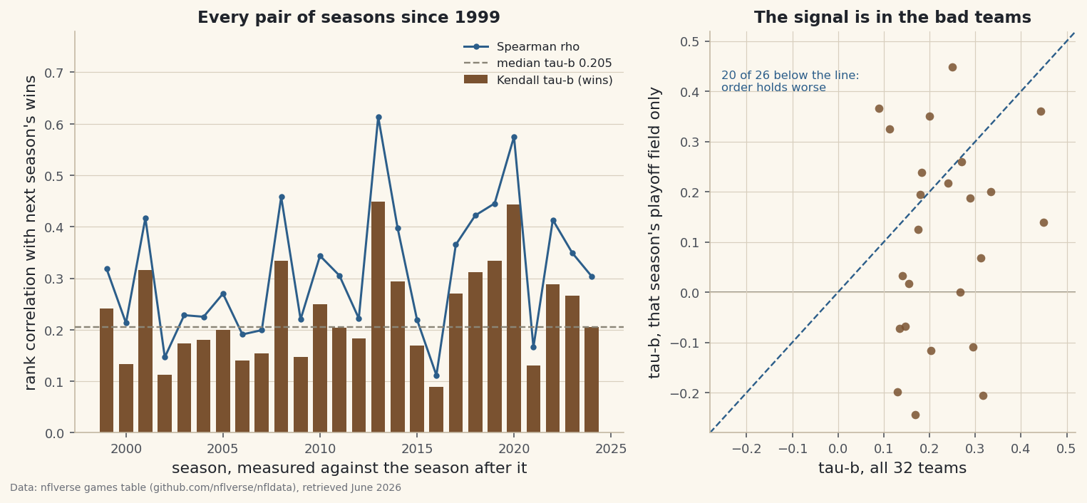
Ask whether one NFL season tells you anything about the next and the reflex is a correlation coefficient: 0.345 between 2023 wins and 2024 wins. That number is a claim about straight lines and distances, which is not what anyone argues about. The argument is about order — who finished above whom — and order has its own coefficient. Kendall’s tau counts pairs of teams. Of the 417 pairs whose 2023 finish was unambiguous, 269 kept their order in 2024 and 148 flipped: 64.51%, against the 50% a coin would give. Written by hand below that comes out as tau-b = 0.2668, and across all 26 consecutive pairs of seasons since 1999 the median is 0.2049 with every single pair positive. The persistence is small, real, and relentless. Then restrict the same measurement to the teams that actually reached the playoffs and it evaporates — median 0.0963, positive in only 16 of 26, and the 2023 field landing on exactly zero: 35 concordant pairs against 35 discordant.

Bring the correlation and regression tutorial, because this is the same question asked without the line, and the percentiles tutorial, because everything here happens in rank space. Everything runs offline from the bundled nfl_games_lines.csv — every game since 1999 with scores, trimmed from the nflverse games table (June 2026 snapshot) — with one cross-check against the bundled NHL file at the end. No scipy, no pandas .corr shortcuts for the ranks.

1. One row per team-season, and a look at what ties

   The file has one row per game, so a team’s season is the rows where it appears on either side. Stack home and away, fold the three franchises that changed city, and count. A tie game is half a win, which matters more here than it looks: it is one of the reasons two teams end a season level. Before choosing a method, ask the data how often it refuses to order two teams at all.

   import pandas as pd
   import numpy as np
   
   FRANCHISE = {"STL": "LA", "SD": "LAC", "OAK": "LV"}   # a move is not a new team
   
   games = pd.read_csv("nfl_games_lines.csv")
   reg = games[(games.game_type == "REG") & games.result.notna()]
   
   sides = []
   for me, opp in (("home", "away"), ("away", "home")):
       s = reg[["season", f"{me}_team", f"{me}_score", f"{opp}_score"]].copy()
       s.columns = ["season", "team", "pf", "pa"]
       sides.append(s)
   tg = pd.concat(sides, ignore_index=True)
   tg["team"] = tg.team.replace(FRANCHISE)
   tg["w"] = (tg.pf > tg.pa) + 0.5 * (tg.pf == tg.pa)     # a tie is half a win
   
   ts = (tg.groupby(["season", "team"])
           .agg(gp=("w", "size"), wins=("w", "sum"), pf=("pf", "sum"), pa=("pa", "sum"))
           .reset_index())
   ts["pdiff"] = ts.pf - ts.pa
   print(len(games), "rows ->", len(reg), "played games ->", len(ts), "team-seasons")

   861 team-seasons, and a column that cannot order 7.81% of its pairs

   7548 rows in the file -> 6967 played regular-season games -> 861 team-seasons, 1999-2025
     tie games kept as half a win: 15
     teams per season: 31 (1999-2001) to 32 (Houston arrives in 2002)
     games per team: 16 through 2020, 17 from 2021 - except 2022, where BUF, CIN played 16
   
   within-season pairs of teams, 1999-2025: 13299
     tied on wins:              1039  (7.81%)
     tied on point differential:  40  (0.30%)
   ties are the whole reason this page has two versions of Kendall's tau.

   Two things in that output decide everything that follows. The first is the schedule: 16 games per team through 2020, 17 from 2021, and one odd season in 2022 where Buffalo and Cincinnati played 16 because a game was abandoned. Raw win totals are therefore not comparable across seasons, and a rank method never asks them to be — it only ever compares two teams inside the same season. The second is the tie rate. Across 13,299 within-season pairs of teams, 1,039 are level on wins, 7.81%, while only 40 pairs are level on point differential, 0.30%. A method that pretends ties do not happen is going to have an opinion about one pair in thirteen.

2. Count the pairs

   The whole method is a loop over pairs. Take two teams: if the season that just ended and the season that follows agree about which is better, the pair is concordant; if they disagree, it is discordant. Kendall’s tau-a is the difference between those counts over the number of pairs there are, so it runs from −1 to +1 and reads as a net share of pairs that held. To see it work with no complications, take a group with no ties anywhere: the six best point differentials of 2005, and the same six teams in 2006.

   import math
   import itertools
   
   def pair_counts(x, y):
       C = D = Tx = Ty = Txy = 0
       for i in range(len(x)):
           for j in range(i + 1, len(x)):
               a, b = np.sign(x[i] - x[j]), np.sign(y[i] - y[j])
               if a == 0 and b == 0: Txy += 1      # tied on both
               elif a == 0:          Tx += 1       # tied on x only
               elif b == 0:          Ty += 1       # tied on y only
               elif a * b > 0:       C += 1        # concordant
               else:                 D += 1        # discordant
       return C, D, Tx, Ty, Txy
   
   def tau_a(x, y):
       C, D, _tx, _ty, _txy = pair_counts(x, y)
       n = len(x)
       return (C - D) / (n * (n - 1) / 2)
   
   prev = ts[ts.season == 2005].set_index("team").pdiff.sort_values(ascending=False).head(6)
   teams = list(prev.index)
   x = prev.to_numpy(float)
   y = ts[ts.season == 2006].set_index("team").loc[teams, "pdiff"].to_numpy(float)
   
   # the exact null: every relabeling of the second column, all 720 of them
   null = np.array([tau_a(x, y[list(p)]) for p in itertools.permutations(range(6))])
   print(tau_a(x, y), null.std(), (np.abs(null) >= abs(tau_a(x, y))).mean())

   Fifteen pairs, ten of them concordant, and a null you can enumerate completely

   the six best point differentials of 2005, and the same teams in 2006 (point differential almost never ties):
   
     team   2005   2006
     IND     +192    +67
     SEA     +181     -6
     DEN     +137    +14
     CAR     +132    -35
     PIT     +131    +38
     NYG     +108     -7
   
   every one of the 15 pairs, classified:
      IND  vs SEA   2005   +11   2006   +73   concordant
      IND  vs DEN   2005   +55   2006   +53   concordant
      IND  vs CAR   2005   +60   2006  +102   concordant
      IND  vs PIT   2005   +61   2006   +29   concordant
      IND  vs NYG   2005   +84   2006   +74   concordant
      SEA  vs DEN   2005   +44   2006   -20   discordant
      SEA  vs CAR   2005   +49   2006   +29   concordant
      SEA  vs PIT   2005   +50   2006   -44   discordant
      SEA  vs NYG   2005   +73   2006    +1   concordant
      DEN  vs CAR   2005    +5   2006   +49   concordant
      DEN  vs PIT   2005    +6   2006   -24   discordant
      DEN  vs NYG   2005   +29   2006   +21   concordant
      CAR  vs PIT   2005    +1   2006   -73   discordant
      CAR  vs NYG   2005   +24   2006   -28   discordant
      PIT  vs NYG   2005   +23   2006   +45   concordant
   
     concordant 10, discordant 5, tied 0
     tau-a = (10 - 5) / 15 = 0.333333
   
   is a third of a tau worth anything at n = 6? Enumerate the whole null:
     720 relabelings of the second column, every one of them
     distinct values of tau-a: 16
     null mean 0.000000000000, null sd 0.354860
     the no-ties formula says the sd should be 0.354860
     exact P(tau >= 0.3333) = 0.234722, two-sided 0.469444
   six teams cannot tell you anything. The arithmetic is still the arithmetic.

   The arithmetic is small enough to check by eye. Indianapolis had the best differential of 2005 and the best of 2006, so its five pairs are all concordant. Seattle beat Denver in 2005 and lost to it in 2006, so that pair is discordant. Ten pairs held and five flipped, giving tau-a = (10 − 5) / 15 = 0.3333. Then comes the part worth more than the coefficient. With six teams you can write down the entire null distribution — all 720 relabelings of the second column — and ask how often chance alone produces a third of a tau. The answer is 23.47% one-sided, 46.94% two-sided. Nothing has been demonstrated. The enumeration also pays a dividend: its standard deviation is 0.354860, and the textbook formula for the null spread of tau-a returns 0.354860 as well. With no ties present that formula is not an approximation at all, which is exactly why the next step is about ties.

3. What ties do, and the correction that answers them

   Now use wins, where ties are everywhere. The four teams that reached the 2023 conference championship games make the problem visible at a glance: Detroit and San Francisco both won 12 in 2023, and Detroit and Kansas City both won 15 in 2024. Those pairs are not concordant and not discordant. They are unorderable, and tau-a quietly charges them to the denominator anyway. Kendall’s 1945 repair, tau-b, divides instead by what each column can actually order, dropping from each side separately the pairs that side cannot rank.

   def tau_b(x, y):
       C, D, Tx, Ty, _txy = pair_counts(x, y)
       return (C - D) / math.sqrt((C + D + Tx) * (C + D + Ty))
   
   prev = ts[ts.season == 2023].set_index("team")
   nxt = ts[ts.season == 2024].set_index("team")
   both = sorted(set(prev.index) & set(nxt.index))
   X, Y = prev.loc[both, "wins"].to_numpy(float), nxt.loc[both, "wins"].to_numpy(float)
   
   print(pair_counts(X, Y))
   print("tau-a", tau_a(X, Y), " tau-b", tau_b(X, Y))
   print("against itself:", tau_a(X, X), tau_b(X, X))   # perfect agreement

   Four teams by hand, then 496 pairs: tau-a 0.2440 against tau-b 0.2668

   the four teams that reached the 2023 conference championship games, by regular-season wins:
   
     team   2023  2024
     BAL      13    12
     DET      12    15
     KC       11    15
     SF       12     6
   
     concordant 1, discordant 3, tied on 2023 only 1, tied on 2024 only 1, tied on both 0
     tau-a = (1 - 3) / 6            = -0.333333
     tau-b = (1 - 3) / sqrt(5 x 5) = -0.400000
   
   the whole league, 2023 wins against 2024 wins (32 teams, 496 pairs):
     concordant 269, discordant 148
     tied on 2023 only 42, on 2024 only 31, on both 6 -> 79 pairs no order at all
     of the 417 pairs both seasons DO order, 64.51% kept their order
   
     tau-a 0.243952   tau-b 0.266833
   
     the clearest way to see why tau-b exists: score the 2023 column against ITSELF.
       perfect agreement by construction, and tau-a still reads 0.903226,
         because 48 of the 496 pairs are tied inside that one column
       tau-b reads 1.000000
   tau-b divides by what each column can actually order.
   That is the only difference, and it is why tau-b is the one to quote.

   For the four-team group, one pair held, three flipped, one is tied on 2023 and one on 2024. Tau-a reports (1 − 3) / 6 = −0.3333; tau-b divides the same −2 by √(5 × 5) and reports −0.4000. Across the full league the correction runs the other way, lifting 0.2440 to 0.2668, because 79 of the 496 pairs are unorderable by one season or the other.

   The clearest demonstration of why the correction exists is the last line of that output, where I score the 2023 column against itself. That is perfect agreement by construction, and tau-a still reads 0.9032, because 48 pairs are tied inside the column and tau-a counts them as failures to agree. Tau-b reads exactly 1. A coefficient that cannot reach 1 when a ranking is compared with a copy of itself is not measuring what its name promises. One caution the symmetry hides: tau-b reaches 1 only when both columns carry the same tie groups, so it is not a magic restoration of the full range either.

4. Spearman’s rho, and the shortcut that does not survive ties

   The other classical answer is older. Spearman’s rho, from 1904, replaces each value with its rank and runs an ordinary correlation on those. Ties share the average of the ranks they span. Every textbook also gives a shortcut, 1 − 6∑d² / (n(n²−1)), which is algebraically identical to the definition — and identical only when nothing is tied.

   def midranks(v):
       v = np.asarray(v, dtype=float)
       order = v.argsort()
       r = np.empty(len(v)); r[order] = np.arange(1, len(v) + 1)
       for u in np.unique(v):                     # tied values share their average rank
           m = v == u
           if m.sum() > 1:
               r[m] = r[m].mean()
       return r
   
   def spearman_rho(x, y):
       return float(np.corrcoef(midranks(x), midranks(y))[0, 1])
   
   def spearman_shortcut(x, y):
       n = len(x)
       d = midranks(x) - midranks(y)
       return 1 - 6 * float((d ** 2).sum()) / (n * (n * n - 1))
   
   print(spearman_rho(X, Y), spearman_shortcut(X, Y), np.corrcoef(X, Y)[0, 1])

   The shortcut overstates rho in 26 of 26 season pairs, never once below

   the same 2023 -> 2024 table, three coefficients:
   
     Kendall tau-b (pairs that kept their order)  0.266833
     Spearman rho  (Pearson on the midranks)      0.349467
     Pearson r     (on the raw win totals)        0.345234
   
   rho and tau-b are not rivals and not on the same scale: tau-b is a share of pairs,
   rho is a correlation of ranks. rho is reliably the larger number.
   
   the textbook shortcut 1 - 6*sum(d^2)/(n(n^2-1)) on the same column: 0.359421
     that is +0.009954 away from rho, because it is only equal to Pearson-on-ranks when nothing is tied.
   
   across all 26 consecutive-season pairs:
     season   rho      shortcut   gap
     2006   0.1910   0.2068   +0.0158
     2002   0.1467   0.1600   +0.0133
     2005   0.2702   0.2832   +0.0130
     1999   0.3184   0.3314   +0.0129
     ...
     the shortcut is ABOVE the real value in 26 of 26 pairs, never below, by at most 0.015791
   a one-directional error is a bias, not a rounding difference.
   Compute rho as Pearson on the midranks.

   On the 2023 table rho is 0.3495 and the shortcut returns 0.3594, too high by 0.0099. That gap is not rounding. Run both across all 26 season pairs and the shortcut comes out above the real value 26 times out of 26, never once below, by as much as 0.0158 in 2006. An error with a consistent sign is a bias, and since ties are guaranteed in win totals, the shortcut is simply the wrong formula for this column. Compute rho as Pearson on the midranks and the problem disappears.

   It is worth saying what rho and tau-b are not. They are not competitors for the same number and they do not share a scale: tau-b is a net share of pairs, rho is a correlation of rank positions, and rho is reliably the larger of the two. Quoting one as though it were the other is the most common way this pair of methods gets misused.

5. Twenty-six season pairs, and whether any one of them is real

   One season pair is an anecdote. Run the same measurement on every consecutive pair since 1999 and the shape of the answer appears, along with the question of whether a single year’s value can be distinguished from zero at all. The classical test is a normal approximation built on the null variance of C − D — derived, as it happens, assuming no ties. The honest alternative is the permutation test: shuffle one column and recompute.

   def tau_normal_z(x, y):
       C, D, _tx, _ty, _txy = pair_counts(x, y)
       n = len(x)
       return 3 * (C - D) / math.sqrt(n * (n - 1) * (2 * n + 5) / 2)
   
   z = tau_normal_z(X, Y)
   print("normal z", z, "two-sided p", math.erfc(abs(z) / math.sqrt(2)))
   
   rng = np.random.default_rng(96)
   obs = tau_b(X, Y)
   null = np.array([tau_b(X, rng.permutation(Y)) for _ in range(10000)])
   print("shuffled p", (np.abs(null) >= abs(obs)).mean())

   Every pair positive, median tau-b 0.2049, and one season that lands on p = 0.0497

   every consecutive pair of seasons, 1999-2025:
   
     season   n   tau-a   tau-b     rho   Pearson
     1999   31  0.2194  0.2409  0.3184   0.3609
     2000   31  0.1247  0.1341  0.2131   0.1884
     2001   31  0.2925  0.3166  0.4170   0.3807
     2002   32  0.1028  0.1127  0.1467   0.1849
     2003   32  0.1593  0.1742  0.2284   0.2423
     2004   32  0.1653  0.1798  0.2253   0.2596
     2005   32  0.1815  0.1998  0.2702   0.2860
     2006   32  0.1270  0.1406  0.1910   0.2616
     2007   32  0.1411  0.1544  0.1993   0.2095
     2008   32  0.3105  0.3341  0.4579   0.5693
     2009   32  0.1351  0.1473  0.2202   0.2306
     2010   32  0.2258  0.2492  0.3437   0.3752
     2011   32  0.1875  0.2037  0.3054   0.2752
     2012   32  0.1694  0.1834  0.2221   0.1779
     2013   32  0.4153  0.4493  0.6137   0.5926
     2014   32  0.2742  0.2944  0.3976   0.3783
     2015   32  0.1593  0.1692  0.2198   0.2710
     2016   32  0.0827  0.0889  0.1117   0.2594
     2017   32  0.2500  0.2708  0.3652   0.3502
     2018   32  0.2923  0.3118  0.4220   0.4119
     2019   32  0.3125  0.3341  0.4453   0.4556
     2020   32  0.4133  0.4437  0.5750   0.6402
     2021   32  0.1210  0.1303  0.1661   0.2255
     2022   32  0.2641  0.2883  0.4134   0.3730
     2023   32  0.2440  0.2668  0.3495   0.3452
     2024   32  0.1915  0.2061  0.3039   0.2840
   
     median   tau-a 0.1895   tau-b 0.2049   rho 0.3046   Pearson 0.2850
     tau-b is positive in 26 of 26 pairs, from 0.0889 (2016) to 0.4493 (2013)
   
   is one season's tau-b distinguishable from zero? Take 2023:
     normal approximation  z = 1.9622, two-sided p = 0.04974
     10000 shuffles   two-sided p = 0.04750
     null sd of tau-a: 0.124572 shuffled, 0.124326 from the no-ties formula
   
   at n = 32 the tie correction to the null barely matters (79 tied pairs of 496).
   at n = 4, where 2 of 6 pairs are tied, the same formula claims sd 0.4907 and the exact enumeration says 0.4357.

   Tau-b is positive in 26 of 26 pairs, with a median of 0.2049, a low of 0.0889 (2016 into 2017) and a high of 0.4493 (2013 into 2014). The medians for the other coefficients — tau-a 0.1895, rho 0.3046, Pearson 0.2850 — sit where the previous step said they would. Twenty-six positives in twenty-six independent draws would be overwhelming evidence on its own, and I would not lean on it too hard, because consecutive pairs share a season each and are not independent.

   For a single year the two tests agree: 2023 gives z = 1.9622 and p = 0.0497 from the normal approximation against 0.0475 from ten thousand shuffles, which is one season scraping past a threshold it has no business being judged by. They agree because the tie correction to the null barely bites at this size: the shuffled spread of tau-a is 0.1246 against the formula’s 0.1243. Shrink the problem and the agreement collapses. For the four-team group from step three, where two of six pairs are tied, the formula claims a null spread of 0.4907 and complete enumeration says 0.4357. The approximation does not know ties exist, and at small n that is the difference between a p-value and a guess.

6. Where the persistence actually lives

   A median tau-b of 0.205 across the league invites the obvious follow-up: is that order being kept at the top, where the interesting teams are? Restrict the measurement to the teams that made the playoffs in the first season — a group the file defines for itself, no arbitrary cutoff required — and measure the same thing.

   playoffs = games[games.game_type.isin(["WC", "DIV", "CON", "SB"]) & games.result.notna()]
   
   for yr in range(1999, 2025):
       d = playoffs[playoffs.season == yr]
       field = sorted(set(d.home_team.replace(FRANCHISE)) | set(d.away_team.replace(FRANCHISE)))
       a = ts[ts.season == yr].set_index("team")
       b = ts[ts.season == yr + 1].set_index("team")
       f = [t for t in field if t in a.index and t in b.index]
       print(yr, len(f), round(tau_b(a.loc[f, "wins"].to_numpy(float),
                                     b.loc[f, "wins"].to_numpy(float)), 4))

   Median tau-b falls from 0.2049 league-wide to 0.0963 inside the playoff field

   restrict the same measurement to the teams that made the playoffs that season:
   
     full league     median tau-b 0.2049   positive in 26 of 26
     playoff field   median tau-b 0.0963   positive in 16 of 26
     the field is the lower of the two in 20 of 26 pairs
   
     2023's 14 playoff teams, into 2024: concordant 35, discordant 35, tied 21 -> tau-b +0.0000
   
   does last season's point differential order next season better than its wins do?
   
     median tau-b from wins              0.2049
     median tau-b from point differential 0.2227
     point differential wins 17 of the 26 head-to-heads, sign-test two-sided p = 0.1686
     (the two orders agree within a season at a median tau-b of 0.7741, so they are mostly the same ranking)
   
   one season pair from another sport, for scale - NHL points, 2024-25 into 2025-26:
     tau-b 0.1423   rho 0.2096   Pearson 0.2191   two-sided p 0.2632

   The median falls from 0.2049 to 0.0963, the count of positive pairs falls from 26 of 26 to 16 of 26, and the field is the lower of the two in 20 of 26 seasons. The 2023 playoff field is the cleanest illustration available: 35 concordant pairs, 35 discordant, tau-b exactly zero. This is range restriction doing what range restriction does, and it is the same phenomenon the regression-to-the-mean tutorial measures from the other side. Most of what makes a season predict the next one is the bottom of the table staying at the bottom. Among teams that were all good, next year’s order is close to a fresh draw.

   One more comparison, because it is the claim every analyst repeats: point differential is supposed to predict next season better than the record does. By this measurement it does, barely — median tau-b 0.2227 against 0.2049 — and it wins 17 of the 26 head-to-heads, which a sign test puts at p = 0.1686. That is not a result. The two orderings are mostly the same ranking anyway, agreeing within a season at a median tau-b of 0.7741, so there was never much room between them. For scale from another sport, the bundled NHL file gives one season pair — points in 2024-25 against 2025-26 — at tau-b 0.1423, rho 0.2096, two-sided p 0.2632, which is a single pair and settles nothing on its own; the PDO tutorial reads those same two seasons with Pearson correlations.

   

Where this breaks

Six limits. Rank correlation only sees order. A season where the best team wins 17 and a season where it wins 11 are the same ranking, so tau cannot tell you that the league compressed; that is a question for the raw numbers and for a regression. Wins are a coarse ranking. Seventeen games produce heavy ties, and 7.81% of within-season pairs are level; tau-b handles them honestly but cannot invent information the schedule never produced. The 26 pairs are not independent. Each season appears in two of them, so “26 of 26 positive” is weaker evidence than a binomial count would suggest, and I have not attempted a correction for it. The normal approximation ignores ties, which is harmless at 32 teams and badly wrong at four; enumerate or shuffle whenever the group is small. Playoff qualification is not a clean cut. The field is chosen partly by division, so restricting to it does not restrict cleanly to the best teams, and some of the collapse in step six is that ragged boundary rather than pure range restriction. And none of this explains anything. Persistence of order is compatible with stable rosters, stable coaching, stable ownership and an unequal schedule, and this page separates none of them.

Sources. Games and scores: the nflverse games table, June 2026 snapshot, bundled by build/make_nfl_lines_csv.py as nfl_games_lines.csv; attribution to nflverse required. NHL points: the NHL public API, retrieved August 2026, bundled as nhl_team_pdo_two_seasons.csv. The coefficient: M. G. Kendall, “A New Measure of Rank Correlation,” Biometrika 30(1-2), 1938, pp. 81-93, doi:10.1093/biomet/30.1-2.81. The tie correction: M. G. Kendall, “The Treatment of Ties in Ranking Problems,” Biometrika 33(3), 1945, pp. 239-251, doi:10.1093/biomet/33.3.239. The older coefficient: C. Spearman, “The Proof and Measurement of Association between Two Things,” The American Journal of Psychology 15(1), 1904, pp. 72-101, doi:10.2307/1412159. Every number on this page is recomputed by the tutorial’s script, whose asserts fail rather than print a figure they cannot reproduce.

Troubleshooting