Predict a Scoreline with Poisson: the World Cup Final as a Grid

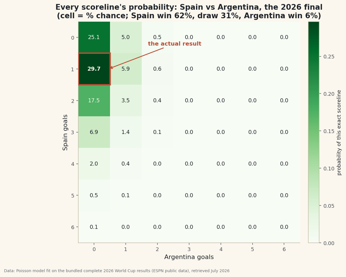
Every bookmaker's correct-score market, every FiveThirtyEight-style match forecast, and half the football-analytics industry rests on one idea small enough to fit in a tweet: goals arrive like radioactive decay. A goal is a rare event that can happen at any moment of a match, so the number of goals a team scores follows a Poisson distribution — and once you buy that, a whole match becomes a multiplication: P(Spain scores h) × P(Argentina scores a) for every pair, laid out as a grid where every possible scoreline has a probability. This tutorial builds that model from scratch — the pmf hand-written in math, no scipy, no fitting library — on the completed 2026 World Cup, all 104 matches. The payoff is genuinely eerie: the model's single most likely cell for the final is Spain 1-0, at 29.7% — and Spain 1-0 is exactly how the real final ended.

Just as important, we'll check the model the honest way at both ends: first whether World Cup goals actually follow a Poisson distribution (almost — and the way it misses teaches the model's next refinement), and last where the multiplication itself breaks (it under-predicts draws, measurably, and for a footballing reason). You met this dataset in the goals-by-stage tutorial, which owns the stage-by-stage story; here the same 104 matches become a forecasting machine. Everything runs offline on the bundled wc2026_results.csv, it's pure numpy/pandas/math, and there's no randomness anywhere — every number recomputes identically on every run.

1. One number first: the tournament's goal rate

   A Poisson distribution is fully described by a single parameter, λ (lambda) — the average number of events per interval. Our event is a goal, our interval is one team's ninety-ish minutes. So reshape the file from one row per match to one row per team per match — 104 matches become 208 scoring opportunities — and take the mean.

   import math
   import numpy as np
   import pandas as pd
   
   df = pd.read_csv("wc2026_results.csv")
   long = pd.concat([
       pd.DataFrame({"team": df["home"], "scored": df["home_goals"],
                     "conceded": df["away_goals"]}),
       pd.DataFrame({"team": df["away"], "scored": df["away_goals"],
                     "conceded": df["home_goals"]}),
   ], ignore_index=True)
   
   lam0 = long["scored"].mean()
   print(len(df), len(long), round(lam0, 3), round(long["scored"].var(ddof=1), 3))

   The tournament in two moments: mean and variance

   104 matches -> 208 team-matches
   
     goals per team per match (lambda)   1.481
     variance of goals per team-match    1.942
     variance / mean                     1.31
   
   a Poisson variable's variance EQUALS its mean, so that ratio should
   be ~1.00. we got 1.31 - our first hint that one shared rate is too
   simple. hold the thought; first, how close does one rate get?

   1.481 goals per team per match. But the variance line is the first real finding: a Poisson variable's variance equals its mean — that's not a rule of thumb, it's a theorem — and ours is 31% too big. Remember from the distributions tutorial what excess variance means: the data is more spread out than one single-rate process can explain. File that away; step 2 shows exactly where it bites.

2. The honest check: do World Cup goals actually look Poisson?

   Before trusting the model with a forecast, make it pass a lineup. Write the Poisson probability mass function yourself — it's one line — and stand its predicted goal counts next to the 208 real ones. Then score the comparison with the chi-square machinery you built in the chi-square tutorial: six bins (0, 1, 2, 3, 4, 5+), and because we estimated λ from this same data we give up one extra degree of freedom, leaving df = 4 and a 5% critical value of 9.488.

   def pois(k, lam):
       return math.exp(-lam) * lam ** k / math.factorial(k)
   
   obs = long["scored"].value_counts().reindex(range(8), fill_value=0)
   expected = np.array([len(long) * pois(k, lam0) for k in range(8)])
   
   obs_b = list(obs[:5]) + [int(obs[5:].sum())]
   exp_b = list(expected[:5]) + [len(long) - expected[:5].sum()]
   chi2 = sum((o - e) ** 2 / e for o, e in zip(obs_b, exp_b))
   print(round(chi2, 2))

   Observed goal counts vs one shared Poisson rate

   goals scored by one team in one match - observed vs Poisson(1.481):
   
      goals   observed   Poisson expects
        0         55           47.3
        1         71           70.1
        2         39           51.9
        3         25           25.6
        4         10            9.5
        5          5            2.8
        6          2            0.7
        7          1            0.1
   
   close - the shape is unmistakably Poisson-ish - but look at the
   misses: too many 0s (55 vs 47), too few 2s (39 vs 52), too many
   blowout tallies of 5+. pooling bins 0-4 and 5+:
   
     chi-square = 9.57  vs the df=4, 5% bar of 9.488
   
   a hair over the line. the single-rate model fails, and for a
   physical reason: 48 different teams don't share one lambda. mixing
   strong and weak attacks fattens both tails - that's the var/mean of
   1.31 showing up again. the fix is one rate per team.

   9.57 against a bar of 9.488 — the single-rate model fails, by a whisker, and the pattern of the misses is the diagnosis. Too many zeros, too few twos, too many 5-goal-plus tallies: that's the signature of a mixture. Spain's matches don't run at the same λ as Panama's, and pooling strong attacks with weak ones fattens both tails — the same fact the 1.31 variance ratio was shouting in step 1. One chart holds the whole verdict:

   import matplotlib.pyplot as plt
   
   fig, ax = plt.subplots(figsize=(9.6, 5.2))
   ax.bar(range(8), obs, color="#2E7D4F", label="observed (208 team-matches)")
   ax.plot(range(8), expected, color="#20242B", marker="o",
           label="Poisson, one shared rate")
   ax.set_xlabel("goals scored by one team in one match")
   ax.legend()
   fig.savefig("goals_fit.png", dpi=144, bbox_inches="tight")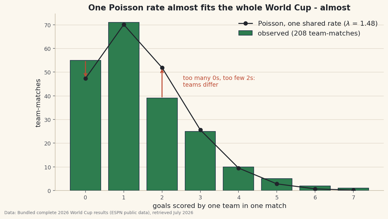

   

   Read the chart generously and skeptically at once: the shape is unmistakably Poisson-like — this is why the model family is the industry standard — but the misfit is real, and it points directly at the fix. Don't give the tournament one λ. Give every team its own.

3. Attack and defence multipliers for all 48 teams

   The classic parameterization is multiplicative. Each team gets an attack rate (goals scored per match, relative to the tournament's 1.481) and a defence rate (goals conceded per match, same scale — lower is better). An average team is 1.000 on both dials. Because every 2026 venue was neutral for all but three teams, we skip the home-advantage multiplier a league model would need — one honest simplification, declared.

   rates = long.groupby("team").agg(games=("scored", "size"),
                                    scored=("scored", "mean"),
                                    conceded=("conceded", "mean"))
   rates["attack"] = rates["scored"] / lam0
   rates["defence"] = rates["conceded"] / lam0
   print(rates.sort_values("attack", ascending=False).head(4).round(3))

   The tournament's sharpest attacks and stingiest defences

   attack = goals scored per match / 1.481   (1 = tournament average)
   defence = goals conceded per match / 1.481 (lower = stingier)
   
   sharpest attacks:
                games  scored  conceded  attack  defence
   team                                                 
   Netherlands      4    2.75      1.25   1.857    0.844
   Germany          4    2.75      1.25   1.857    0.844
   England          8    2.50      1.50   1.688    1.013
   France           8    2.50      1.25   1.688    0.844
   
   stingiest defences:
             games  scored  conceded  attack  defence
   team                                              
   Spain         8    1.75     0.125   1.182    0.084
   Colombia      5    1.00     0.200   0.675    0.135
   Portugal      5    1.60     0.600   1.081    0.405
   Mexico        5    2.00     0.600   1.351    0.405
   
   Spain conceded ONCE in eight games - defence 0.084. and note the
   games column: finalists played 8, group-stage exits played 3.
   Panama scored 0 goals in 3 games, so their attack multiplier is
   0.000 - the model now claims Panama can literally never score.
   three games of evidence, taken at face value. remember that.

   The table passes the sniff test — the four semifinalists all show up with elite numbers, and Spain's defence multiplier of 0.084 encodes a real fact: one goal conceded in eight games. But look hard at the games column and at Panama. Sixteen teams played only three matches, and Panama's zero goals in three games produce an attack multiplier of exactly 0.000 — this model now asserts Panama could never, ever score. That's not a bug in our code; it's what taking 3-game samples at face value means. The regression-to-the-mean tutorial showed you the cure (shrink extreme small-sample rates toward the average); here, just carry the caveat visibly.

4. The score matrix: every scoreline, priced

   Now the machine assembles. For a fixture, expected goals for each side are tournament rate × my attack × your defence. Take the final — Spain vs Argentina — and turn each side's λ into a probability for scoring 0, 1, 2… goals. The key modeling assumption, worth saying out loud because step 5 will test it: the two sides' goal counts are independent, so every scoreline's probability is a plain product, and np.outer builds all 49 cells at once. Spain's win probability is the sum below the diagonal, the draw is the diagonal's trace, Argentina's is the rest.

   lam_h = lam0 * rates.loc["Spain", "attack"] * rates.loc["Argentina", "defence"]
   lam_a = lam0 * rates.loc["Argentina", "attack"] * rates.loc["Spain", "defence"]
   
   K = 7
   p_h = np.array([pois(k, lam_h) for k in range(K)])
   p_a = np.array([pois(k, lam_a) for k in range(K)])
   M = np.outer(p_h, p_a)          # M[h, a] = P(Spain h) * P(Argentina a)
   
   print(np.unravel_index(M.argmax(), M.shape), round(M.max(), 3))
   print(round(np.tril(M, -1).sum(), 3), round(np.trace(M), 3),
         round(np.triu(M, 1).sum(), 3))

   The final as the model saw it: lambdas, top scorelines, win/draw/loss

   the final, Spain vs Argentina:
   
     lambda_Spain     = 1.481 x 1.182 x 0.675 = 1.18 expected goals
     lambda_Argentina = 1.481 x 1.604 x 0.084 = 0.20 expected goals
   
   most likely scorelines:
       Spain 1-0  29.7%
       Spain 0-0  25.1%
       Spain 2-0  17.5%
       Spain 3-0  6.9%
       Spain 1-1  5.9%
   
     Spain win  62.3%   draw  31.4%   Argentina win  6.2%
     (the 7x7 grid holds 100.0% of all probability)
   
   the model's top cell is 1-0 Spain. the real final: Spain 1-0.

   Sit with that output for a second. The model hands Argentina — twice recently world champions, 2.375 goals a game in this tournament — an expected-goals number of 0.20, because their attack meets a defence multiplier of 0.084. It calls Spain 1-0 the most likely exact score at 29.7%, with 0-0 second at 25.1%, and prices the match at 62.3% Spain, 31.4% draw, 6.2% Argentina. The real final finished Spain 1-0. Enjoy the shiver, then keep your head: hitting the modal scoreline is partly skill (Spain really were that stingy) and partly fortune — even the model itself said its best guess lands only three times in ten. The grid, drawn:

   fig, ax = plt.subplots(figsize=(8.6, 7.0))
   ax.imshow(M, cmap="Greens")
   for i in range(K):
       for j in range(K):
           ax.text(j, i, f"{M[i, j] * 100:.1f}", ha="center", va="center")
   ax.set_xlabel("Argentina goals")
   ax.set_ylabel("Spain goals")
   fig.savefig("score_matrix.png", dpi=144, bbox_inches="tight")

   

   This grid is the actual product bookmakers sell as a correct-score market, and it composes: sum any region and you've priced a bet. Under 2.5 goals? Add the cells where h + a < 3. Both teams to score? Everything off the first row and column. And if you want match odds turned into tournament odds, the score matrix is exactly the per-game engine you'd plug into the Monte Carlo season simulator or the best-of-seven machinery.

5. Where independence breaks: the missing draws

   The multiplication in step 4 assumed Spain's goal count tells you nothing about Argentina's. Football knows better — teams respond to the scoreboard — and the place the assumption fails is famous enough to have a named fix. Measure it: run the model over all 72 group games (the only stage where a draw can stand), sum each game's diagonal, and compare with the draws that actually happened.

   grp = df[df["stage"] == "group"]
   drawn = (grp["home_goals"] == grp["away_goals"]).sum()
   
   exp_draws = 0.0
   for _, m in grp.iterrows():
       lh = lam0 * rates.loc[m["home"], "attack"] * rates.loc[m["away"], "defence"]
       la = lam0 * rates.loc[m["away"], "attack"] * rates.loc[m["home"], "defence"]
       exp_draws += sum(pois(k, lh) * pois(k, la) for k in range(7))
   
   print(drawn, round(exp_draws, 1))

   Draws: what independence predicts vs what happened

   run the model over all 72 group games (the only stage that can end
   level) and add up each game's draw probability:
   
     draws the model expects   15.1
     draws that happened       20
   
   the shortfall is systematic, not bad luck: multiplying the two
   Poissons assumes the sides score INDEPENDENTLY, but real teams
   respond to the scoreboard - level games tighten up, 1-1 protects
   itself. every serious scoreline model patches exactly this cell
   (Dixon & Coles, 1997); the patch is the challenge below.

   Twenty draws happened; independence expected 15.1. One tournament can't make that gap definitive — the shortfall is within shouting distance of chance — but it points exactly where forty years of fitting this model to whole leagues points: real matches produce more low-scoring draws (0-0, 1-1) than the product of two Poissons allows, because level games tighten up and protect the point. Dixon & Coles (1997) patched precisely these four cells with a small correlation adjustment, and their correction is still inside most professional scoreline models. You now know why it exists — you measured the hole it fills.

What this model is, and what it isn't

You've built the industry's baseline, and its honest edges are as instructive as its hits. First, the sample is tiny by design: 104 matches price the tournament's average well, but per-team multipliers rest on 3–8 games each — which is how Panama's attack became literally zero and why Spain's 0.084 defence, extrapolated forever, would be absurd. Club-season versions of this model feast on 380 matches of a league with every team playing 38; a World Cup is the hard mode. Second, we fit on the tournament we then "predicted" — fine for teaching the machinery, and the troubleshooting entry below shows the honest held-out version barely differs here, but a real forecast only ever uses matches played before kickoff. Third, knockout games that went to extra time are recorded here with their full-game goal totals — a slightly longer "interval" for λ than the group games' ninety minutes; a production model would rate goals per minute. None of this dents the core: a hand-built Poisson grid, honestly checked, that put its biggest single bet on the exact final score.

Troubleshooting