Principal Component Analysis: Where a Box Score Hides Its Shooting

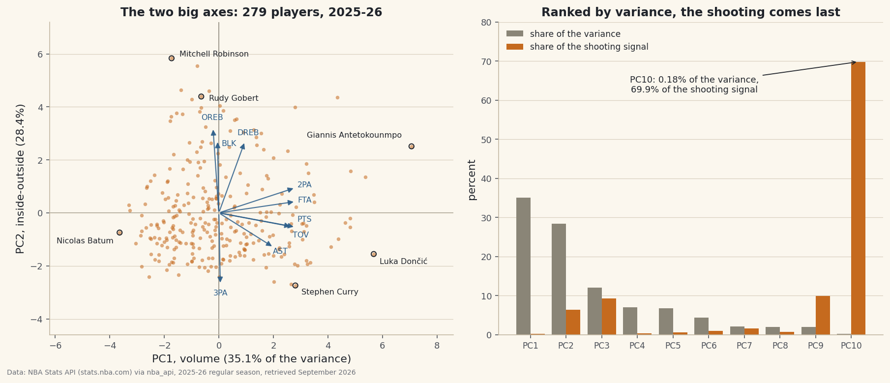
Ten numbers per 36 minutes describe every NBA player who logged at least 1,000 minutes in 2025-26: points, two- and three-point attempts, free-throw attempts, offensive and defensive rebounds, assists, turnovers, steals and blocks. Principal component analysis asks how many independent numbers that line really holds, and for these 279 players the answer is two big ones and a small third. The first component is volume, how much of the offence a player carries: 35.1% of the variance, and its scores correlate +0.910 with the league’s usage rate, a column the analysis never saw. The second is inside-outside, rebounds and blocks against threes and assists: 28.4%. A shuffled-noise test keeps a third, mostly steals. The inside-outside axis is also steadier than any single stat in the table: it repeats from one season to the next at a median correlation of .968, and beats every one of the ten stats it is built from in all 21 season pairs since 2004-05. The surprise is at the other end. The component PCA ranks last carries 0.18% of the variance and 69.9% of the shooting signal, the points a player scores beyond what his attempts would yield at average conversion rates. Compress the ten numbers to the top three components, the usual move, and Stephen Curry’s +2.48 points per 36 of shooting becomes −0.23. Ranked by variance, the shooting comes last.

Bring the z-scores tutorial, because PCA starts from standardized columns, and the correlation-heatmap tutorial, because the matrix PCA takes apart is the one that heatmap draws. K-means was this course’s first look at data with no labels; this is the second. Everything runs offline from the bundled nba_player_seasons.csv, one row per player per regular season from 2004-05 to 2025-26, pulled from the NBA’s own stats API (stats.nba.com) with nba_api. No scikit-learn: the components come from power iteration, under twenty lines of numpy, and numpy’s own eigensolver appears only to check them.

1. Ten rates per 36 minutes, standardized

   Totals reward playing time, so every count becomes a rate per 36 minutes, and a 1,000-minute floor keeps players whose rates rest on a real sample. Two-point attempts are field-goal attempts minus threes, so the two kinds of shot get separate columns. Then each column is standardized: subtract its mean, divide by its standard deviation.

   import numpy as np
   import pandas as pd
   
   df = pd.read_csv("nba_player_seasons.csv")
   df["fg2a"] = df.fga - df.fg3a                       # two-point attempts
   STATS = ["pts", "fg2a", "fg3a", "fta", "oreb", "dreb", "ast", "tov", "stl", "blk"]
   COLS = [s + "36" for s in STATS]
   for s in STATS:
       df[s + "36"] = 36 * df[s] / df["min"]           # every count as a rate per 36 minutes
   
   d = df[(df.season == "2025-26") & (df["min"] >= 1000)].reset_index(drop=True)
   X = d[COLS].to_numpy(float)
   mu, sd = X.mean(axis=0), X.std(axis=0)
   Z = (X - mu) / sd                                   # z-scores: every column mean 0, sd 1
   R = Z.T @ Z / len(Z)                                # their covariance is the correlation matrix
   print(len(df), len(d))
   print(pd.Series(sd ** 2 / (sd ** 2).sum(), index=COLS).round(3))   # share of the raw variance

   279 of 582 players qualify; points alone hold 45.7% of the raw variance

   bundled file: 11,059 player-seasons, 22 seasons (2004-05 to 2025-26)
   2025-26 regular season: 582 players, 279 with 1,000+ minutes
   per 36 minutes            mean      sd   share of the raw variance
   points                  17.510   5.186    45.7%
   2-pt attempts            7.854   3.245    17.9%
   3-pt attempts            5.540   2.672    12.1%
   free-throw attempts      3.552   2.036     7.0%
   off. rebounds            1.705   1.230     2.6%
   def. rebounds            4.859   1.835     5.7%
   assists                  3.958   2.022     7.0%
   turnovers                2.046   0.774     1.0%
   steals                   1.268   0.441     0.3%
   blocks                   0.732   0.589     0.6%
   standardized: every column has mean 0 and sd 1, so each holds 10% of the variance

   The last column is why the standardizing matters. PCA hunts for the directions in which the data spreads most, and in raw units points per 36 spread far more than anything else: an sd of 5.186 against 0.441 for steals, 45.7% of all the raw variance against 0.3%. Fed raw rates, PCA would mostly rediscover points, and step three shows it doing exactly that. After standardizing, every column has a variance of 1 and the same 10% claim on the total, so the components have to be built from how the stats move together, not from their units. The covariance of z-scores is the correlation matrix, the same table a correlation heatmap colours in, and that ten-by-ten matrix is the whole input to everything below.

2. Two columns first: PCA on paper

   With two standardized columns the whole analysis can be done by hand. Their correlation matrix is [[1, r], [r, 1]], its eigenvalues are 1 + r and 1 − r, and its eigenvectors are (1, 1)/√2 and (1, −1)/√2, the two 45-degree lines, whatever r is. The eigenvalue is the variance along that direction; the eigenvector is the direction. Offensive rebounds and blocks per 36 make a good pair: both are things that happen near the basket.

   import math
   
   r = R[4, 9]                              # offensive rebounds with blocks, per 36
   C2 = np.array([[1, r], [r, 1]])          # the 2 x 2 correlation matrix
   print("r", r, "eigenvalues", 1 + r, 1 - r, "PC1 share", (1 + r) / 2)
   
   q = (1 - r) / (1 + r)
   v = np.array([1.0, 0.0])                 # start anywhere; here, all offensive rebounds
   for k in range(1, 7):
       v = C2 @ v                           # multiply by the matrix...
       v /= np.linalg.norm(v)               # ...and rescale to length one
       angle = math.degrees(math.atan2(v[1], v[0]))
       print(k, v.round(5), round(angle, 3), math.tan(math.radians(45 - angle)), q ** k)

   The gap to 45 degrees shrinks by q = 0.26805 a step, exactly

   offensive rebounds vs blocks per 36, 279 players: r = 0.5772
   eigenvalues 1 + r = 1.5772 and 1 - r = 0.4228; PC1 holds (1 + r) / 2 = 78.86%
   eigenvectors (0.7071, 0.7071) and (0.7071, -0.7071): the two 45-degree lines
   power iteration from (1, 0); q = (1 - r) / (1 + r) = 0.26805
   step  vector               angle   gap to 45   tan(gap)   q^step
      1  (0.86607, 0.49992)  29.995     15.005    0.26805   0.26805
      2  (0.75596, 0.65461)  40.890      4.110    0.07185   0.07185
      3  (0.72059, 0.69336)  43.897      1.103    0.01926   0.01926
      4  (0.71075, 0.70345)  44.704      0.296    0.00516   0.00516
      5  (0.70808, 0.70613)  44.921      0.079    0.00138   0.00138
      6  (0.70737, 0.70684)  44.979      0.021    0.00037   0.00037

   The correlation is 0.5772, so the first component of this pair holds (1 + r)/2 = 78.86% of its variance, and the second the rest. The loop is power iteration, the method that will find all ten components in the next step. Start from any vector, multiply it by the matrix, rescale it to length one, and repeat. Written in the eigenvector directions, the start (1, 0) has equal parts along each; every multiplication stretches the first part by 1 + r = 1.5772 and the second by 1 − r = 0.4228, so the second part shrinks relative to the first by q = 0.4228/1.5772 = 0.26805 a step. That gives an exact prediction: after k steps the tangent of the remaining gap to 45 degrees is q^k. The output checks it. After one step the vector sits at 29.995 degrees, a gap of 15.005 whose tangent is 0.26805; after two, at 40.890, a tangent of 0.07185 = q²; after four, within 0.296 degrees. The lesson carries over: power iteration converges at the rate of the second eigenvalue over the first, so two components of nearly equal size take a long time to tell apart.

3. Ten columns: power iteration, then deflation

   The same loop on the ten-by-ten matrix finds the top component. To find the next, remove the one just found: subtracting λvv^T from the matrix leaves every other eigenpair untouched and sets this one’s eigenvalue to zero, so the next run of power iteration lands on the second-largest. Ten rounds of that, called deflation, give all ten components in order.

   def power_iteration(A, tol=1e-12, max_iter=100_000):
       v = np.random.default_rng(0).normal(size=len(A))   # a random start
       v /= np.linalg.norm(v)
       for it in range(1, max_iter + 1):
           w = A @ v
           w /= np.linalg.norm(w)
           if np.abs(w - v).max() < tol:
               return w @ A @ w, w, it                     # eigenvalue, eigenvector, steps
           v = w
       raise RuntimeError("power iteration did not converge")
   
   def pca_by_hand(A):
       A = A.copy()
       vals, vecs, iters = [], [], []
       for _ in range(len(A)):
           lam, v, it = power_iteration(A)
           vals.append(lam); vecs.append(v); iters.append(it)
           A = A - lam * np.outer(v, v)                    # deflation: remove the pair just found
       return np.array(vals), np.column_stack(vecs), iters
   
   vals, V, iters = pca_by_hand(R)
   share = vals / vals.sum()
   print(vals.round(5), share.round(4), share.cumsum().round(4), iters)
   print("gap to numpy:", np.abs(vals - np.linalg.eigvalsh(R)[::-1]).max())
   
   raw_vals, raw_V, _ = pca_by_hand(np.cov(X, rowvar=False, bias=True))   # unstandardized
   print("raw PC1:", raw_vals[0] / raw_vals.sum(), "loading on points:", abs(raw_V[0, 0]))

   Two components hold 63.46% of the variance; the tenth holds 0.18%

   power iteration with deflation on the 10 x 10 correlation matrix
   component  eigenvalue    share   cumulative   iterations
           1     3.50811   35.08%      35.08%          122
           2     2.83836   28.38%      63.46%           27
           3     1.20765   12.08%      75.54%           59
           4     0.70426    7.04%      82.58%          577
           5     0.67607    6.76%      89.34%           63
           6     0.44242    4.42%      93.77%           36
           7     0.21538    2.15%      95.92%          258
           8     0.19592    1.96%      97.88%         2090
           9     0.19382    1.94%      99.82%           13
          10     0.01801    0.18%     100.00%            2
   eigenvalues sum to 10.000000, the number of standardized columns
   largest gap to numpy.linalg.eigvalsh: 6.7e-16; to the SVD of Z: 4.4e-16
   the same solver on the raw rates: PC1 takes 65.39% of the variance,
     and its loading on points is 0.824

   The eigenvalues add up to 10, the number of standardized columns, because a rotation moves variance around without creating or destroying any. The first component takes 35.08%, the second 28.38%, the third 12.08%, and the first two together 63.46%: ten numbers, most of whose spread lies in a plane. The tenth eigenvalue is 0.01801, almost nothing, and step six is about why. The solver agrees with numpy’s eigvalsh and with the singular value decomposition of Z to within 10⁻¹⁵. The iteration counts repeat the two-column lesson: most components settle within a few hundred steps, but the eighth takes over 2,000, because its eigenvalue, 0.19592, is barely larger than the ninth’s, 0.19382. The last line runs the same solver on the raw, unstandardized rates, and the first component swallows 65.39% of the variance with a loading of 0.824 on points. That is the raw-units trap from step one: the biggest number wins.

4. Read the two big axes

   A component is a direction, and its ten coordinates are called loadings: how much each standardized stat contributes to it. A player’s score on a component is his ten z-scores multiplied by its ten loadings and summed. One convention first. An eigenvector and its negative are equally valid, and solvers return either, so each axis is flipped to make its largest loading positive. Any fixed rule would do; what matters is having one.

   V = V * np.sign(V[np.abs(V).argmax(axis=0), np.arange(10)])   # largest loading positive
   S = Z @ V                                                     # each player's ten scores
   print(pd.DataFrame(V[:, :3], index=COLS, columns=["PC1", "PC2", "PC3"]).round(3))
   print("usage rate:", [round(np.corrcoef(S[:, k], d.usg_pct)[0, 1], 3) for k in range(3)])
   
   d["pc1"], d["pc2"] = S[:, 0], S[:, 1]
   for col in ("pc1", "pc2"):
       print(d.nlargest(3, col)[["player", col]].to_string(index=False))
       print(d.nsmallest(3, col)[["player", col]].to_string(index=False))
   
   i = d.index[d.player == "Stephen Curry"][0]
   print((Z[i] * V[:, 0]).round(4), "sum", (Z[i] * V[:, 0]).sum())   # a score is a dot product

   PC1 is volume, PC2 is inside-outside, PC3 is mostly steals

   loadings, each axis flipped so its largest loading is positive
                              PC1     PC2     PC3
   points                  +0.469  -0.090  -0.289
   2-pt attempts           +0.468  +0.158  -0.025
   3-pt attempts           +0.009  -0.452  -0.307
   free-throw attempts     +0.470  +0.071  -0.124
   off. rebounds           -0.036  +0.536  +0.099
   def. rebounds           +0.160  +0.451  -0.037
   assists                 +0.335  -0.217  +0.402
   turnovers               +0.448  -0.087  +0.221
   steals                  -0.022  -0.060  +0.760
   blocks                  -0.008  +0.457  -0.080
   correlation with the league's usage rate, which is not one of the ten columns:
     PC1 +0.910, PC2 -0.245, PC3 -0.198
   PC1 highest: Giannis Antetokounmpo +7.07, Luka Dončić +5.68, Nikola Jokić +5.38
   PC1 lowest : Nicolas Batum -3.64, Spencer Jones -3.31, Dean Wade -3.27
   PC2 highest: Mitchell Robinson +5.84, Robert Williams III +5.55, Yves Missi +4.64
   PC2 lowest : Stephen Curry -2.74, LaMelo Ball -2.68, Darius Garland -2.59
   worked example, Stephen Curry's PC1 score = his ten z-scores times the PC1 loadings
                                 z   loading   product
   points                  +2.5898   +0.4689   +1.2144
   2-pt attempts           +0.2097   +0.4678   +0.0981
   3-pt attempts           +2.8340   +0.0092   +0.0261
   free-throw attempts     +1.1966   +0.4697   +0.5620
   off. rebounds           -1.0119   -0.0357   +0.0361
   def. rebounds           -0.6250   +0.1597   -0.0998
   assists                 +0.7623   +0.3352   +0.2555
   turnovers               +1.5922   +0.4482   +0.7136
   steals                  +0.1361   -0.0216   -0.0029
   blocks                  -0.4609   -0.0078   +0.0036
   sum                                         +2.8067   (unrounded: +2.8068)

   The first component loads almost equally on points (+0.469), two-point attempts (+0.468), free-throw attempts (+0.470) and turnovers (+0.448), with assists (+0.335) behind them: it measures how much of the offence runs through a player. Its scores correlate +0.910 with the league’s usage rate, a column that was never in the analysis, which is the best evidence the name is right. Giannis Antetokounmpo, Luka Dončić and Nikola Jokić sit at the top; Nicolas Batum, Spencer Jones and Dean Wade sit at the bottom, all three among the five lowest usage rates of the 279. The second component sets offensive rebounds (+0.536), blocks (+0.457) and defensive rebounds (+0.451) against three-point attempts (−0.452) and assists (−0.217): where on the floor a player works. Mitchell Robinson, Robert Williams III and Yves Missi top it, and Stephen Curry, LaMelo Ball and Darius Garland sit at the far perimeter end. The third is mostly steals (+0.760) with assists (+0.402).

   The worked example makes the score concrete. Curry’s PC1 score is the sum of ten products in the output: 2.5898 × 0.4689 = 1.2144 from points, 1.5922 × 0.4482 = 0.7136 from turnovers, 1.1966 × 0.4697 = 0.5620 from free-throw attempts, 0.7623 × 0.3352 = 0.2555 from assists, and small amounts from the other six, for 2.8067 with the rounded inputs and 2.8068 without. His most extreme z-score, +2.8340 for three-point attempts, contributes only +0.0261, because the volume axis gives threes a loading of +0.0092. PC1 counts how many shots a player takes, not where he takes them; where belongs to PC2, on which Curry’s −2.74 is the lowest of the 279.

5. How many components are real?

   Ten components always come out, so the question is how many describe structure rather than chance. The classic answer, usually credited to Kaiser (1960), keeps every component with an eigenvalue above 1, more variance than a single standardized column. A stricter answer is parallel analysis, Horn’s (1965) idea of comparing each eigenvalue with what random data of the same shape produces. Shuffling every column on its own keeps each stat’s values and destroys every relationship between them, the same move as the permutation test. A component is kept if it beats the 95th percentile of its shuffled counterparts, the cut Glorfeld (1995) proposed because Horn’s original, the average, kept too many. Then a second test of a different kind: a component that measures something real about a player should come back the next season.

   def shuffled_eigenvalues(Z, reps, seed):
       rng = np.random.default_rng(seed)
       out = np.empty((reps, Z.shape[1]))
       for i in range(reps):
           Zs = rng.permuted(Z, axis=0)            # shuffle every column on its own
           out[i] = np.linalg.eigvalsh(Zs.T @ Zs / len(Zs))[::-1]
       return out
   
   def parallel_keep(vals, null):
       cut = np.percentile(null, 95, axis=0)       # what chance reaches 5% of the time
       keep = 0
       while keep < len(vals) and vals[keep] > cut[keep]:
           keep += 1
       return keep, cut
   
   print("Kaiser keeps", (vals > 1).sum())
   keep, cut = parallel_keep(vals, shuffled_eigenvalues(Z, 1000, 20261007))
   print("parallel analysis keeps", keep, cut.round(4))
   
   def fit_season(season, min_minutes=1000):
       ds = df[(df.season == season) & (df["min"] >= min_minutes)].reset_index(drop=True)
       Xs = ds[COLS].to_numpy(float)
       Zs = (Xs - Xs.mean(axis=0)) / Xs.std(axis=0)
       w, W = np.linalg.eigh(Zs.T @ Zs / len(Zs))  # numpy's solver, now that ours matches it
       o = np.argsort(w)[::-1]
       w, W = w[o], W[:, o]
       W = W * np.sign(W[np.abs(W).argmax(axis=0), np.arange(10)])
       return ds, Zs, w, W
   
   seasons = sorted(df.season.unique())
   fits = {s: fit_season(s) for s in seasons}
   for s in seasons:
       ds, Zs, w, W = fits[s]
       print(s, round(w[2], 3), parallel_keep(w, shuffled_eigenvalues(Zs, 1000, 20261007))[0])
   
   W26 = fits["2025-26"][3]                        # score every season on the 2025-26 axes
   pers, raw = [], []
   for a, b in zip(seasons[:-1], seasons[1:]):
       (da, Za, _, _), (db, Zb, _, _) = fits[a], fits[b]
       both = np.intersect1d(da.player_id, db.player_id)
       ia = pd.Series(da.index, index=da.player_id)[both].to_numpy()
       ib = pd.Series(db.index, index=db.player_id)[both].to_numpy()
       Sa, Sb = Za[ia] @ W26, Zb[ib] @ W26
       pers.append([np.corrcoef(Sa[:, k], Sb[:, k])[0, 1] for k in range(10)])
       raw.append([np.corrcoef(Za[ia, j], Zb[ib, j])[0, 1] for j in range(10)])
   print(np.median(pers, axis=0).round(3), np.median(raw, axis=0).round(3))

   Kaiser keeps three every season; the shuffles keep three in 12 of 22

   Kaiser's rule (eigenvalue above 1) keeps 3
   parallel analysis, 1,000 shuffles of 2025-26:
   component  eigenvalue  95th pct of shuffled  kept
           1      3.5081                1.3946  yes
           2      2.8384                1.2751  yes
           3      1.2076                1.1884  yes
           4      0.7043                1.1190  no
           5      0.6761                1.0601  no
           6      0.4424                1.0028  no
           7      0.2154                0.9506  no
           8      0.1959                0.8988  no
           9      0.1938                0.8399  no
          10      0.0180                0.7830  no
   22 seasons, 1,000+ minutes: Kaiser keeps 3 in 22; parallel analysis keeps 3 in 12 and 2 in 10
   season   3rd eig  cut   keeps | season   3rd eig  cut   keeps
   2004-05   1.013  1.198    2   | 2015-16   1.129  1.194    2
   2005-06   1.039  1.199    2   | 2016-17   1.292  1.187    3
   2006-07   1.099  1.195    2   | 2017-18   1.196  1.192    3
   2007-08   1.120  1.200    2   | 2018-19   1.254  1.189    3
   2008-09   1.139  1.196    2   | 2019-20   1.300  1.201    3
   2009-10   1.040  1.202    2   | 2020-21   1.344  1.199    3
   2010-11   1.221  1.198    3   | 2021-22   1.296  1.192    3
   2011-12   1.237  1.207    3   | 2022-23   1.320  1.194    3
   2012-13   1.054  1.201    2   | 2023-24   1.225  1.195    3
   2013-14   1.145  1.196    2   | 2024-25   1.207  1.195    3
   2014-15   1.046  1.191    2   | 2025-26   1.208  1.188    3
   next-season persistence on the 2025-26 axes, median r over 21 season pairs
     (177-215 players each):
     PC1 0.897  PC2 0.968  PC3 0.859  PC4 0.778  PC5 0.815
     PC6 0.807  PC7 0.746  PC8 0.798  PC9 0.679  PC10 0.584
     steadiest single stat: off. rebounds 0.942; points 0.872; true shooting % 0.629
     PC2 beats all ten single stats in 21 of 21 pairs; PC1 beats points in 21

   In 2025-26 the two rules agree on three. The first two components clear the shuffled cut easily; the third clears it by a hair, 1.2076 against 1.1884, and the fourth (0.7043 against 1.1190) does not come close. Across all 22 seasons they disagree. Kaiser’s rule keeps three every time, while parallel analysis keeps three in 12 seasons and two in 10: the third component has cleared the noise line in every season since 2016-17 but missed it in 10 of the 12 seasons before. In 2004-05 Kaiser kept a third eigenvalue of 1.013, well short of the 1.198 that one shuffle in twenty reached: the over-keeping Horn’s comparison was designed to catch.

   The persistence test scores every season’s players on the same 2025-26 axes, each season standardized against its own league, and correlates the scores of the players who reached 1,000 minutes in both seasons of each of the 21 consecutive-season pairs, between 177 and 215 players a pair. The inside-outside axis repeats at a median of .968. The steadiest single stat, offensive rebounds, manages .942, and the inside-outside composite beats all ten of its ingredients in every one of the 21 pairs. Averaging several related stats cancels some of each one’s noise, the same reason a longer sample regresses less. The volume axis (.897) beats points per 36 (.872) in all 21 pairs too.

   The small components carry the caution. Components four to nine fail the size test, yet a player’s scores on them repeat at medians from .679 to .815: they are real, stable differences between players, just small ones. Parallel analysis answers whether a direction holds more variance than chance would give it, not whether it means anything, and the clearest case is the component it ranks last.

6. The smallest component is the shooting

   The tenth component loads +0.695 on points and −0.487, −0.438 and −0.270 on two-point, three-point and free-throw attempts, with the other six loadings within 0.099 of zero: it is points against the attempts that produced them. The reason it is so small is an identity. Every point in the file is a two-point make, a three-point make or a free throw (points equal 2 × field goals made + threes made + free throws made on every row, which the script asserts), so points per 36 are almost a fixed function of attempts per 36, and the only freedom left is how well the attempts convert. To measure that freedom directly, compare each player’s points with what his attempts would have scored at the group’s own conversion rates.

   def shooting_points(frame):
       per2 = 2 * (frame.fgm - frame.fg3m).sum() / frame.fg2a.sum()   # points per 2-pt attempt
       per3 = 3 * frame.fg3m.sum() / frame.fg3a.sum()                 # per 3-pt attempt
       perft = frame.ftm.sum() / frame.fta.sum()                      # per free throw
       expected = per2 * frame.fg2a36 + per3 * frame.fg3a36 + perft * frame.fta36
       return (frame.pts36 - expected).to_numpy(), (per2, per3, perft)
   
   print("PC10 loadings", V[:, 9].round(3))
   shot, (per2, per3, perft) = shooting_points(d)
   corr = np.array([np.corrcoef(S[:, k], shot)[0, 1] for k in range(10)])
   print("shares", (corr ** 2).round(4), "total", (corr ** 2).sum())
   
   X3 = mu + sd * (S[:, :3] @ V[:, :3].T)          # every player rebuilt from three numbers
   shot3 = X3[:, 0] - (per2 * X3[:, 1] + per3 * X3[:, 2] + perft * X3[:, 3])
   for p in ("Stephen Curry", "Nikola Jokić", "Bam Adebayo"):
       i = d.index[d.player == p][0]
       print(p, d.pts36[i].round(2), X3[i, 0].round(2), shot[i].round(2), shot3[i].round(2))
   
   for s in seasons:                               # the last component, every season?
       ds, Zs, w, W = fits[s]
       sh, _ = shooting_points(ds)
       c2 = np.array([np.corrcoef(Zs @ W[:, k], sh)[0, 1] for k in range(10)]) ** 2
       print(s, c2.argmax() + 1, c2[9].round(4))
   
   rng = np.random.default_rng(20261007)           # bootstrap: resample the 279 players
   boot_share, boot_gap = [], []
   for _ in range(2000):
       rows = rng.integers(0, len(d), len(d))
       Zb = (X[rows] - X[rows].mean(axis=0)) / X[rows].std(axis=0)
       wb, Wb = np.linalg.eigh(Zb.T @ Zb / len(Zb))   # ascending: column 0 is the smallest
       sb, _ = shooting_points(d.iloc[rows])
       boot_share.append(np.corrcoef(Zb @ Wb[:, 0], sb)[0, 1] ** 2)
       boot_gap.append(wb[-1] - wb[-2])
   print(np.percentile(boot_share, [2.5, 97.5]))

   0.18% of the variance, 69.86% of the shooting signal

   PC10: eigenvalue 0.01801, 0.18% of the variance
     loadings: points +0.695, 2-pt attempts -0.487,
               3-pt attempts -0.438, free-throw attempts -0.270
     the other six loadings are all within 0.099 of zero
   points per 36 regressed on the three attempt rates: R^2 = 0.9543
   group conversion: 1.1053 points per 2-pt attempt, 1.0908 per 3-pt attempt,
     0.7893 per free throw
   shooting points per 36 = points - what those attempts score at those rates (sd 1.134)
   component  share of variance  r with shooting points  share of shooting signal
           1             35.08%                  -0.045                     0.20%
           2             28.38%                  +0.252                     6.36%
           3             12.08%                  -0.304                     9.24%
           4              7.04%                  +0.062                     0.38%
           5              6.76%                  -0.078                     0.61%
           6              4.42%                  -0.098                     0.97%
           7              2.15%                  +0.129                     1.66%
           8              1.96%                  +0.086                     0.75%
           9              1.94%                  -0.316                     9.97%
          10              0.18%                  +0.836                    69.86%
   total                100.00%                                           100.00%
   keep 3 components (75.54% of the variance): 15.80% of the shooting signal survives
                           pts/36  from 3  shooting  from 3
   Stephen Curry            30.94   27.19     +2.48   -0.23
   Nikola Jokić             28.60   27.79     +2.75   -0.39
   Bam Adebayo              22.35   22.07     -1.91   +0.38
   true shooting % vs PC10: r = +0.718
   22 seasons: the last component holds the largest share in 22;
     its share runs 66.2% to 85.3%, its variance never above 0.26%
   2025-26 with other minute floors:
     500+ minutes, 378 players: PC10 holds 71.7%
     1,500+ minutes, 164 players: PC10 holds 73.8%
   bootstrap, 2,000 resamples of the 279 players: PC10's share 57.5% to 76.7%

   Regressing points per 36 on the three attempt rates explains 95.43% of their variance, which is why the leftover is small. The group’s conversion rates are 1.1053 points per two-point attempt, 1.0908 per three and 0.7893 per free throw, and shooting points, the difference between a player’s points and what his attempts were worth at those rates, has a standard deviation of 1.134 per 36. Because shooting points are an exact linear combination of four of the standardized columns, and the ten components are uncorrelated, the squared correlations of shooting points with the ten components add up to exactly 100%, a complete accounting of where the signal sits. The tenth component holds 69.86% of it. The ninth holds 9.97%, the third 9.24%, the second 6.36%, and no other more than 2%.

   That is the cost of the usual compression. Keep the top three components, 75.54% of the variance, and 15.80% of the shooting signal survives. Rebuild each player from his three scores and Curry’s 30.94 points per 36 become 27.19, and his +2.48 points of shooting become −0.23. Jokić’s +2.75 becomes −0.39. Bam Adebayo, 1.91 points per 36 below average conversion, comes back +0.38. A three-number summary keeps each player’s shot volume and replaces his shooting with an average shooter’s. True shooting percentage, which is not a straight combination of the columns, correlates +0.718 with the tenth component.

   None of this is a quirk of one season. In all 22 seasons the last component holds the largest share of the shooting signal, between 66.2% and 85.3%, while never carrying more than 0.26% of the variance; in 2025-26 the share is 71.7% with a 500-minute floor and 73.8% with 1,500. A bootstrap over the 279 players puts it at 57.5% to 76.7%. Jolliffe (1982) made the general point about regression: components with small eigenvalues “can be as important as those with large variance.” It is also the least repeatable component, a median of .584 between seasons against .629 for true shooting percentage itself, because shooting over one season is noisy. Small, important and noisy are three different properties, and PCA’s ordering reports only the first.

7. Do the axes hold still?

   “PC1” is a rank, the direction with the most variance in this sample. Fit the same ten columns in another season and the ranking can change. The season fits from step five already hold every eigenvalue and loading, so the check is short, along with a measure of how far the plane of the first two components moved and the bootstrap gap between their eigenvalues.

   def pc1_kind(W):
       reb, pts = abs(W[4, 0]), abs(W[0, 0])      # offensive rebounds vs points on PC1
       if abs(reb - pts) < 0.01:
           return "blend"
       return "inside-outside" if reb > pts else "volume"
   
   for s in seasons:
       ds, Zs, w, W = fits[s]
       print(s, w[:2].round(3), pc1_kind(W))
   
   P05, P26 = fits["2004-05"][3][:, :2], fits["2025-26"][3][:, :2]
   cosines = np.linalg.svd(P05.T @ P26, compute_uv=False)   # cosines of the angles between planes
   print(cosines.round(3), np.degrees(np.arccos(cosines)).round(1))
   print("gap", vals[0] - vals[1], np.percentile(boot_gap, [2.5, 97.5]))

   The first two components swapped names; the plane they span barely moved

   2004-05: PC1 3.608 = inside-outside: off. rebounds +0.476, def. rebounds +0.433, blocks +0.408,
                                     assists -0.389, 3-pt attempts -0.376
            PC2 2.949 = volume: points +0.511, free-throw attempts +0.490,
                             2-pt attempts +0.482, turnovers +0.466
   2025-26: PC1 3.508 = volume; PC2 2.838 = inside-outside
   what PC1 is, season by season (offensive-rebound vs points loading):
     inside-outside  12  2004-05 to 2015-16
     blend            2  2016-17, 2017-18
     volume           8  2018-19 to 2025-26
   the plane of PC1 and PC2, 2004-05 vs 2025-26:
     principal angles 14.7 and 17.8 degrees (cosines 0.967, 0.952)
   2025-26 gap between the first two eigenvalues: 0.670, bootstrap 95% interval 0.382 to 1.106

   In 2004-05 the first component was the inside-outside axis (eigenvalue 3.608: offensive rebounds +0.476, defensive rebounds +0.433, blocks +0.408 against assists −0.389 and threes −0.376) and the second was volume (2.949). By 2025-26 the order had reversed, volume at 3.508 and inside-outside at 2.838. Classified by whether offensive rebounds or points load harder on it, PC1 was the inside-outside axis in all 12 seasons from 2004-05 to 2015-16, a near-even blend of the two in 2016-17 and 2017-18, and the volume axis in all 8 since 2018-19. The two-dimensional picture changed far less than the labels. The principal angles between the 2004-05 plane and the 2025-26 plane are 14.7 and 17.8 degrees (cosines 0.967 and 0.952), so the same two kinds of difference separate players in both eras; what changed is which of them is larger. In 2025-26 itself the order is not luck: the gap between the first two eigenvalues is 0.670, with a bootstrap interval of 0.382 to 1.106 that stays clear of zero.

   The practical rule follows. Name a component by its loadings, never by its number, and check it in a second sample before building on it. Inside a plane that holds still, the axes can still turn: in 2016-17 and 2017-18 the direction of greatest spread ran between the two familiar ones, so PCA returned blends of both. When two eigenvalues are nearly equal the problem is worse, because the data barely prefers one direction in their plane over another; that is why the eighth component took the solver so long, and why its direction should not be read on its own.

8. Draw the components

   Two pictures carry the argument. A biplot puts every player at his first two scores and draws each stat as an arrow from its loadings, so players sit toward the stats they do most of. Beside it, a bar for each component shows its share of the variance next to its share of the shooting signal.

   import matplotlib.pyplot as plt
   
   fig, (ax1, ax2) = plt.subplots(1, 2, figsize=(12.6, 5.4))
   ax1.scatter(S[:, 0], S[:, 1], s=14, color="#C56A1E", alpha=0.55)
   nudge = {"PTS": (0.3, 0.3), "TOV": (0.3, -0.3)}  # these two arrows nearly coincide
   for j, lab in enumerate(["PTS", "2PA", "3PA", "FTA", "OREB", "DREB", "AST", "TOV", "STL", "BLK"]):
       if np.hypot(V[j, 0], V[j, 1]) < 1 / 6:
           continue                                 # steals barely touch this plane
       x, y = 6 * V[j, 0], 6 * V[j, 1]
       ax1.annotate("", xy=(x, y), xytext=(0, 0), arrowprops=dict(arrowstyle="-|>", color="#2C5E8A"))
       dx, dy = nudge.get(lab, (0.7 * V[j, 0], 0.7 * V[j, 1]))
       ax1.text(x + dx, y + dy, lab, color="#2C5E8A", fontsize=8)
   ax1.set_xlabel("PC1, volume")
   ax1.set_ylabel("PC2, inside-outside")
   
   k = np.arange(1, 11)
   ax2.bar(k - 0.2, 100 * share, width=0.4, color="#8A8577", label="share of the variance")
   ax2.bar(k + 0.2, 100 * corr ** 2, width=0.4, color="#C56A1E", label="share of the shooting signal")
   ax2.set_xticks(k, [f"PC{n}" for n in k])
   ax2.legend()
   fig.tight_layout()
   fig.savefig("pca_box_score.png", dpi=144)

   

   The left panel shows the plane the first two components span. Volume runs left to right and inside-outside bottom to top, so the stars of the volume axis spread along the right edge while Robinson and Rudy Gobert sit at the top and Curry near the bottom. The steals arrow is too short to draw, because steals live on the third component. The right panel is the thesis in one picture: the grey bars, ordered as PCA orders them, fall away from the left, and the tallest orange bar stands over the smallest grey one.

Where this breaks

Six limits. PCA ranks directions by spread, not by importance. That is the whole lesson of step six, and it applies to every use of PCA as compression: a summary built from the top components is a summary of volume and position, and the efficiency information it drops is small in variance not because it is unimportant but because points are nearly determined by attempts. The column list decides the answer. Ten per-36 rates were chosen here; add made shots, percentages or minutes and the components change, and every exact identity among the columns (makes and misses adding up to attempts, say) adds an eigenvalue of zero, as the near-identity between points and attempts added a near-zero one here. Standardizing is a choice too. Z-scores give each stat an equal claim on the variance; on raw rates points take over. Neither version is the correct one, and a third option, weighting stats by how reliably they measure a player, is a different method. Rates per 36 minutes assume a player’s production scales with his minutes, which is least true for players whose minutes come in short or unusual stretches, and the 1,000-minute floor trades sample size for coverage; the tenth component held the largest shooting share at 500 and 1,500 minutes as well, but the other components were not re-examined at those floors. Single axes are less stable than the planes they span. Across seasons the first two components turned inside a nearly fixed plane, through two seasons of blends, and when two eigenvalues are nearly tied, as the eighth and ninth are here, their individual directions are close to arbitrary. Name a component only after checking it in another sample. And PCA describes; it does not explain. The volume axis tracks usage because high-usage players shoot, draw fouls and turn the ball over together, not because PCA knows what usage is.

Sources. Player totals: the NBA Stats API (stats.nba.com; LeagueDashPlayerStats, Base and Advanced, regular-season totals) via nba_api, retrieved September 2026 and bundled by build/make_nba_player_seasons_csv.py as nba_player_seasons.csv; when it was bundled, its games and minutes were checked against Basketball-Reference’s season totals and agree, apart from small minute differences in 2004-05. The method: K. Pearson, “On Lines and Planes of Closest Fit to Systems of Points in Space,” Philosophical Magazine 2(11), 1901, pp. 559-572, doi:10.1080/14786440109462720; H. Hotelling, “Analysis of a Complex of Statistical Variables into Principal Components,” Journal of Educational Psychology 24(6), 1933, pp. 417-441, doi:10.1037/h0071325. Power iteration: R. von Mises and H. Pollaczek-Geiringer, “Praktische Verfahren der Gleichungsauflösung,” Zeitschrift für Angewandte Mathematik und Mechanik 9(1), 1929, pp. 58-77, doi:10.1002/zamm.19290090105. How many components: H. F. Kaiser, “The Application of Electronic Computers to Factor Analysis,” Educational and Psychological Measurement 20(1), 1960, pp. 141-151, doi:10.1177/001316446002000116; J. L. Horn, “A Rationale and Test for the Number of Factors in Factor Analysis,” Psychometrika 30(2), 1965, pp. 179-185, doi:10.1007/BF02289447; L. W. Glorfeld, “An Improvement on Horn’s Parallel Analysis Methodology for Selecting the Correct Number of Factors to Retain,” Educational and Psychological Measurement 55(3), 1995, pp. 377-393, doi:10.1177/0013164495055003002. Small components that matter: I. T. Jolliffe, “A Note on the Use of Principal Components in Regression,” Applied Statistics 31(3), 1982, doi:10.2307/2348005. A modern review: I. T. Jolliffe and J. Cadima, “Principal Component Analysis: A Review and Recent Developments,” Philosophical Transactions of the Royal Society A 374, 2016, 20150202, doi:10.1098/rsta.2015.0202. Every number on this page is recomputed by the tutorial’s script, whose asserts fail rather than print a figure they cannot reproduce.

Troubleshooting