Regression Discontinuity: What a Close Win Is Worth

Every Monday a team that won by a point is filed with the winners and a team that lost by a point with the losers, as if the W told you something the margin does not. Regression discontinuity is the method built to test exactly that. A rule hands out the treatment at a cutoff (finish above zero and you won), so the teams just above the line and the teams just below it should differ in nothing but the treatment, and any jump in what happens to them next is the treatment’s doing. We ran it on every decided regular-season NFL game from 1999 to 2025, from both sides: 13,904 team-games, 13,043 of them followed by another game that season. A close win buys nothing we can measure. At the one-score bandwidth the next week’s win rate jumps by +2.9 points with a 95% interval of −2.9 to +9.0, the next week’s closing line by +0.23 points and the margin against that line by −0.43, and all three intervals straddle zero. What does jump is the one thing the method says cannot: the line the game itself was played at. At the cutoff, narrow winners had gone in as 0.604-point favourites and narrow losers as 0.604-point underdogs, a gap of +1.21 points (95% interval +0.26 to +2.15) that holds at every bandwidth from 9 up, survives dropping the overtime games and is larger than all 21 placebo cutoffs we tried. The closest NFL games are not quite coin flips.

Bring the bootstrap tutorial, because every interval here comes from resampling whole games, and the regression-to-the-mean tutorial, because a one-point result is mostly noise and that piece measures how much. Everything runs offline from the bundled nfl_games_lines.csv (every game since 1999 with scores and the closing line, trimmed from the nflverse games table, June 2026 snapshot) and a new companion file, nfl_games_overtime.csv, which adds the same snapshot’s overtime flag game by game. No scipy, no statsmodels, no rdrobust: each local line is five weighted sums.

1. Two rows per game, and a cutoff at zero

   A regression discontinuity needs three things: a running variable, a cutoff on it that decides who is treated, and an outcome measured afterwards. Here the running variable is a team’s own final margin, the cutoff is zero and the treatment is the W. Every game becomes two rows, one per side, so a three-point home win is a row at +3 for the home team and a row at −3 for the visitors. The outcome is what the same team did in its next game of that regular season. The closing line is turned to each team’s point of view, so it reads as the points that team was favoured by; the point-spread tutorial shows how well that one number forecasts a game.

   import numpy as np
   import pandas as pd
   
   games = pd.read_csv("nfl_games_lines.csv")
   ot = pd.read_csv("nfl_games_overtime.csv")
   games = games.merge(ot, on="game_id", how="left", validate="one_to_one")
   reg = games[(games.game_type == "REG") & games.result.notna()]
   
   sides = []
   for me, sign, venue in (("home", 1, 1), ("away", -1, -1)):
       sides.append(pd.DataFrame({
           "game_id": reg.game_id, "season": reg.season, "gameday": reg.gameday,
           "team": reg[f"{me}_team"],
           "margin": sign * reg.result,         # the running variable: own final margin
           "line": sign * reg.spread_line,      # points this team was favoured by
           "venue": np.where(reg.location == "Home", venue, 0),
           "overtime": reg.overtime}))
   tg = (pd.concat(sides, ignore_index=True)
           .sort_values(["team", "season", "gameday"], kind="stable").reset_index(drop=True))
   
   by = tg.groupby(["team", "season"], sort=False)
   tg["next_margin"] = by.margin.shift(-1)      # the same team's next regular-season game
   tg["next_line"] = by.line.shift(-1)
   tg["next_win"] = np.where(tg.next_margin.isna(), np.nan,
                             (tg.next_margin > 0) + 0.5 * (tg.next_margin == 0))
   tg["next_cover"] = tg.next_margin - tg.next_line
   
   dec = tg[tg.margin != 0].reset_index(drop=True)            # decided games, both sides
   out = dec[dec.next_margin.notna()].reset_index(drop=True)  # ...whose team plays again
   counts = dec.margin.value_counts()
   print(len(dec), dec.game_id.nunique(), len(out))
   print("mirror:", all(counts[m] == counts.get(-m, 0) for m in counts.index))

   13,904 decided rows, a perfect mirror, and margins that bunch at 3 and 7

   regular-season games played 1999-2025: 6,967
     ties: 15, every one after overtime; overtime games in all: 415
   rows, one per team per game: 13,934
     decided games, both sides:  13,904 rows from 6,952 games
     rows whose team plays again that regular season: 13,043
     rows with no next game: 861 (429 games where neither side plays again, 3 where one side does not)
   running variable = own final margin, cutoff = 0, treated = won
     decided by 8 points or fewer: 50.75%; by exactly 3 or 7: 24.17%
     rows at +m equal rows at -m for every m: True

   Two choices in that output are deliberate. The first is the sample. Only regular-season games count, and only a next game in the same regular season, because in the playoffs only the winner plays again, and in the last week of the regular season whether a team plays again depends on whether it reached the playoffs, which depends on the very game being studied. Either way the treatment would decide who stays in the data. The 861 rows with no next game are the 429 final-week games, where neither side plays again, and three week-16 games from 1999 to 2001, when a 31-team league meant one team sat out the final week. The schedule settled every one of them before kickoff.

   The second is the mirror. Because each game contributes +m and −m, the count of rows at +3 equals the count at −3 for every margin. The standard check for a gamed cutoff is a jump in the density of the running variable there (McCrary 2008), and with both sides of every game in the data it passes by construction. A check that cannot fail tells us nothing, so step five uses one that can. The margins are lumpy, too: 50.75% of decided games end within eight points and 24.17% by exactly 3 or 7, and the local lines will be drawn through those lumps.

2. Look at the cells beside the cutoff

   Before fitting anything, look. Group the rows by margin and read the cells on either side of zero: the share of next games won, the line the market posted for that next game, and, from every decided row, the line the game itself was played at.

   cells = out[out.margin.abs() <= 3].groupby("margin").agg(
       rows=("next_win", "size"), next_win=("next_win", "mean"),
       next_line=("next_line", "mean"))
   cells["pre_line"] = dec[dec.margin.abs() <= 3].groupby("margin").line.mean()
   print(cells.round(4))

   One-point winners won 52.15% of their next games, one-point losers 44.24%

   margin  rows  next-game win %  next-game line | pre-game line (all rows)
      -3    993           50.15          -0.19  | -1.0315 (1046)
      -2    263           44.49          -0.90  | -0.9321 (287)
      -1    278           44.24          -0.61  | -0.7594 (293)
      +1    279           52.15          -0.08  | +0.7594 (293)
      +2    263           50.38          +0.59  | +0.9321 (287)
      +3    994           50.00          +0.25  | +1.0315 (1046)

   The rows either side of zero look like a finding. Teams that won by one won 52.15% of their next games and teams that lost by one won 44.24%, a gap of 7.91 points. At two points the gap is 5.89. At three it is −0.15, and the three-point cells hold 994 and 993 rows, more than the one- and two-point cells put together. Either the effect lives only in the very closest games or it is noise in cells of 263 to 279 rows, and the eye cannot settle which. The last column is the one to keep. One-point winners had been favoured by 0.7594 points before kickoff and one-point losers were underdogs by exactly as much, because they are the same 293 games seen from the two sides.

3. Fit a straight line on each side, by hand

   The estimate is the gap between two lines at the cutoff: fit one line to the rows just right of zero and another to the rows just left of it, and read both at zero. Two choices define the fit. The bandwidth h sets how far from zero a game can finish and still count; the kernel sets how much it counts. We use triangular weights, 1 − |m|/h, so a one-point game counts most and a game at the edge of the window least, and h = 9, which admits every one-score game, margins 1 to 8, at weights from 8/9 down to 1/9. The line itself is ordinary weighted least squares, solved from five sums.

   def wls_line(x, y, w):
       """Weighted least-squares line y = a + b*x, from five weighted sums."""
       s0, sx, sxx = w.sum(), (w * x).sum(), (w * x * x).sum()
       sy, sxy = (w * y).sum(), (w * x * y).sum()
       b = (s0 * sxy - sx * sy) / (s0 * sxx - sx * sx)
       return (sy - b * sx) / s0, b
   
   def side_line(x, y, h, right, freq=None):
       keep = ((x > 0) if right else (x < 0)) & (np.abs(x) < h) & ~np.isnan(y)
       w = 1 - np.abs(x[keep]) / h                # triangular: most weight at the cutoff
       if freq is not None:
           w = w * freq[keep]                     # bootstrap counts, used in step four
       return wls_line(x[keep], y[keep], w)
   
   def rd_jump(x, y, h, freq=None):
       return side_line(x, y, h, True, freq)[0] - side_line(x, y, h, False, freq)[0]
   
   H = 9                                          # margins 1-8: every one-score game
   x_out, x_dec = out.margin.to_numpy(float), dec.margin.to_numpy(float)
   y_line = dec.line.to_numpy(float)
   for col, scale in (("next_win", 100), ("next_margin", 1), ("next_line", 1), ("next_cover", 1)):
       print(col, rd_jump(x_out, scale * out[col].to_numpy(float), H))
   print("pre-game line", rd_jump(x_dec, y_line, H))
   print("worked example, h = 4:", rd_jump(x_dec, y_line, 4))

   The worked example by hand, then the bandwidth-9 table, where one jump stands out

   worked example: pre-game line, winning side, bandwidth 4
   margin  rows  sum of lines  mean line  kernel  rows x kernel
        1   293         222.5    0.75939     3/4         219.75
        2   287         267.5    0.93206     1/2         143.50
        3  1046        1079.0    1.03155     1/4         261.50
   weighted mean margin 5165/2499 = 2.06683, weighted mean line 1521/1666 = 0.91297
   slope 0.13535 per point -> line at zero 0.91297 - 0.13535 x 2.06683 = +0.63322
   mirror: the losing side ends at -0.63322, jump +1.26645 (row-by-row fit: +1.26645)
   
   bandwidth 9: margins 1-8 each side, weights 8/9 down to 1/9
                            just above 0 just below 0     jump
   next-game win rate             48.955       46.055   +2.900
   next-game margin               -1.052       -0.849   -0.203
   next-game line                 -0.217       -0.448   +0.232
   next-game cover margin         -0.836       -0.401   -0.435
   pre-game line                   0.604       -0.604   +1.209

   The output opens with the arithmetic done small enough to check, on the pre-game line at h = 4. With whole-number margins, a weighted fit through the rows is the same as a fit through the three cell means, each weighted by its rows times its kernel weight: 293 × 3/4 = 219.75, 287 × 1/2 = 143.5 and 1,046 × 1/4 = 261.5, a total of 624.75. The three-point cell gets the smallest kernel weight and still carries 41.86% of the total, because three is the most common final margin in the file. The weighted means are a margin of 5165/2499 = 2.06683 and a line of 1521/1666 = 0.91297, the weighted slope is 0.13535 points of line per point of margin, and the line at zero is 0.91297 − 0.13535 × 2.06683 = 0.63322. The mirror finishes the job: the losing side is the same games, so its line ends at −0.63322, and the jump is twice that, 1.26645, exactly what the row-by-row fit returns.

   At the working bandwidth the same calculation runs over eight cells a side. The next-game win rate is 48.955% just above zero and 46.055% just below, a jump of +2.90 points. The next game’s margin jumps by −0.203, its closing line by +0.232 and the margin against that line, the cover, by −0.435; the first is the sum of the other two, and the script checks that it is. The odd one out is the last row. The pre-game line jumps by +1.209: at the cutoff, narrow winners had been 0.604-point favourites and narrow losers 0.604-point underdogs. Nothing that happens in a game can change the line it was played at, so this jump cannot be an effect of winning. Step five takes it seriously.

4. Resample whole games, then move the window

   A jump without an interval is a guess. The bootstrap supplies one, with one change: the unit we resample is the game, not the row. A game’s two rows are tied together (in the pre-game line they are exact negatives of each other), so resampling rows one at a time would treat one game as two independent facts and make the interval too narrow. Drawing 6,952 games with replacement is the same as giving each game a random count, 0, 1, 2 and so on, and using that count as a weight, which is how the code does it. Then the same jump goes through six bandwidths.

   code_of = {g: i for i, g in enumerate(pd.unique(dec.game_id))}
   dec_code = dec.game_id.map(code_of).to_numpy()
   out_code = out.game_id.map(code_of).to_numpy()
   G = len(code_of)
   y_win = 100 * out.next_win.to_numpy(float)
   
   rng = np.random.default_rng(20261004)
   boot_win, boot_line = [], []
   for _ in range(2000):
       # G games drawn with replacement = a count per game, used as a weight,
       # so a game's winner row and loser row always travel together
       counts = np.bincount(rng.integers(0, G, G), minlength=G).astype(float)
       boot_win.append(rd_jump(x_out, y_win, H, freq=counts[out_code]))
       boot_line.append(rd_jump(x_dec, y_line, H, freq=counts[dec_code]))
   print(np.percentile(boot_win, [2.5, 97.5]), np.percentile(boot_line, [2.5, 97.5]))
   
   for h in (4, 6, 9, 12, 16, 22):               # one jump, six windows
       print(h, rd_jump(x_out, y_win, h), rd_jump(x_dec, y_line, h))

   Every next-week interval straddles zero; the pre-game line's does not

   bandwidth 9, 2,000 bootstrap resamples of 6,952 games
                                jump   95% interval
   next-game win rate         +2.900   -2.947 to +8.987
   next-game margin           -0.203   -1.851 to +1.538
   next-game line             +0.232   -0.429 to +0.928
   next-game cover margin     -0.435   -1.920 to +1.115
   pre-game line              +1.209   +0.265 to +2.149
   
   bandwidth  next-game win rate (pts)   next-game cover (pts)    pre-game line (pts)
           4  +12.47 ( +0.46 to +25.28)  +0.81 (-2.26 to +3.94)  +1.27 (-0.65 to +3.21)
           6   +7.84 ( -1.61 to +17.74)  -0.07 (-2.41 to +2.34)  +1.14 (-0.32 to +2.67)
           9   +2.90 ( -2.95 to  +8.99)  -0.43 (-1.92 to +1.12)  +1.21 (+0.26 to +2.15)
          12   +1.71 ( -3.22 to  +6.67)  -0.58 (-1.85 to +0.67)  +1.16 (+0.35 to +1.96)
          16   +1.11 ( -3.00 to  +5.32)  -0.58 (-1.62 to +0.48)  +1.14 (+0.45 to +1.85)
          22   +1.35 ( -2.20 to  +4.99)  -0.51 (-1.44 to +0.43)  +1.12 (+0.52 to +1.72)

   At bandwidth 9, every next-week interval straddles zero: win rate −2.947 to +8.987 points, margin −1.851 to +1.538, line −0.429 to +0.928, cover −1.920 to +1.115. The pre-game line’s does not: +0.265 to +2.149.

   The sweep is where a discontinuity analysis is easiest to fool. At h = 4, which uses only margins 1 to 3, the next-week jump is +12.47 points with an interval of +0.46 to +25.28, clear of zero. Report that window alone and you have a momentum effect. Widen it and the effect melts: +7.84 at 6, +2.90 at 9, +1.71 at 12, +1.11 at 16 and +1.35 at 22, with every one of those intervals straddling zero. The narrow estimate is a straight line through three noisy cell means a side, and the step-two table shows what it extrapolates from: two small cells with big gaps and one big cell with none. A real effect of winning would not vanish the moment four- to eight-point games are let in, and six windows are six chances for one of them to clear a 5% bar, the trap the multiple-comparisons tutorial measures. The cover margin, which nets out what the market already knew about both teams, never jumps at any window. The pre-game line jumps by between +1.12 and +1.27 at every window, and its interval clears zero at every window from 9 up.

5. The check that matters: what was settled before kickoff

   A discontinuity design earns the word causal only if the cases on either side of the cutoff were alike before the treatment, and that is checkable. Anything fixed before kickoff should be continuous at zero, so run the same fit with a pre-game variable as the outcome. A jump there is not an effect of winning; it says the winners and the losers were different teams going in. We check four such variables, then try to explain the one that jumps.

   tg["pts"] = (tg.margin > 0) + 0.5 * (tg.margin == 0)
   by = tg.groupby(["team", "season"], sort=False)
   tg["winpct_before"] = 100 * (by.pts.cumsum() - tg.pts) / by.cumcount()   # NaN in week one
   tg["prev_margin"] = by.margin.shift(1)
   dec = tg[tg.margin != 0].reset_index(drop=True)          # same rows, two new columns
   
   for col in ("line", "winpct_before", "prev_margin", "venue"):
       print(col, rd_jump(x_dec, dec[col].to_numpy(float), H))
   
   no_ot = (dec.overtime == 0).to_numpy()
   print("without overtime", rd_jump(x_dec[no_ot], y_line[no_ot], H))
   early = (dec.season <= 2011).to_numpy()
   print("1999-2011", rd_jump(x_dec[early], y_line[early], H),
         "2012-2025", rd_jump(x_dec[~early], y_line[~early], H))
   
   # placebo cutoffs: pretend the cutoff sits at 9.5, 10.5, ... 29.5 on the winning side
   win = x_dec > 0
   placebo = np.array([rd_jump(x_dec[win] - c, y_line[win], H) for c in np.arange(9.5, 30.0, 1.0)])
   print(placebo.mean(), placebo.std(ddof=1), np.abs(placebo).max())

   Two pre-game measures jump at zero; overtime, era and the method do not explain it

   pre-determined variable at the cutoff (bandwidth 9)   jump   95% interval
     pre-game line, points                        +1.209   +0.265 to +2.149
     season win % before the game                 +3.527   +0.265 to +6.697
     margin in the previous game                  +0.962   -0.740 to +2.661
     venue (+1 home, -1 away)                     +0.079   -0.085 to +0.238
   games decided by one point: 293; favourite won 159, underdog won 133, pick'em 1
     a fair coin gives the favourite 159+ of 292 with probability 0.0717
   
   is it overtime, or one era?
     without the overtime games                   +1.124   +0.125 to +2.126
     1999-2011 only                               +2.033   +0.473 to +3.567
     2012-2025 only                               +0.548   -0.626 to +1.750
     difference between the eras +1.485, bootstrap sd 0.994 (1.49 sd)
   
   placebo cutoffs at 9.5, 10.5, ... 29.5 (21 of them), same bandwidth:
     mean jump -0.096, sd 0.427, largest |jump| 0.965; intervals excluding zero: 0
     the real cutoff: +1.209

   The pre-game line jumps by +1.209. The season record coming in says the same thing without the market’s help: narrow winners had won 3.527 percentage points more of their earlier games that season (interval +0.265 to +6.697). The previous week’s margin points the same way, +0.962, but its interval, −0.740 to +2.661, includes zero. Venue does not jump (+0.079, interval −0.085 to +0.238), so narrow winners were not simply at home more often.

   The raw counts lean the same way, more weakly. Of the 293 games decided by one point the favourite won 159, the underdog won 133 and one was a pick’em. On its own that is thin: a fair coin hands the favourite 159 or more of 292 with probability 0.0717. The fitted lines pool every margin out to eight points and find the tilt with more precision.

   We tested three explanations. Overtime is the obvious one, since the better team may win the extra period more often, but dropping all 400 decided overtime games leaves the jump at +1.124 (interval +0.125 to +2.126). Era is the second: the jump is +2.033 in 1999-2011 and +0.548 in 2012-2025, which looks like a story until the difference, +1.485, is set against its bootstrap spread of 0.994. That is 1.49 standard deviations, so we do not claim the tilt has faded. The third suspect is the method: perhaps local lines through lumpy margins manufacture jumps wherever they are pointed. So we moved the cutoff to 21 places where nothing changes hands, 9.5 through 29.5 on the winning side, and ran the identical fit, the same idea as the shuffled null in the permutation-test tutorial. The placebo jumps average −0.096 with a standard deviation of 0.427, the largest is 0.965 in size, and none of their intervals excludes zero. The real cutoff’s +1.209 is larger than all 21.

   This is the pattern Caughey and Sekhon found in close U.S. House elections, where the bare winners were usually the candidates predicted to win. The closest NFL games are sorted too, slightly: the team that was better going in wins a few more of them than a smooth margin allows. For the next-week question the imbalance cuts in one direction. Narrow winners were the stronger teams, which should push their next-week win rate, margin and line up, and those jumps still came back inside the noise. The cover margin is untouched by it, because the line already prices both teams, and it shows nothing at all.

6. Draw the discontinuity

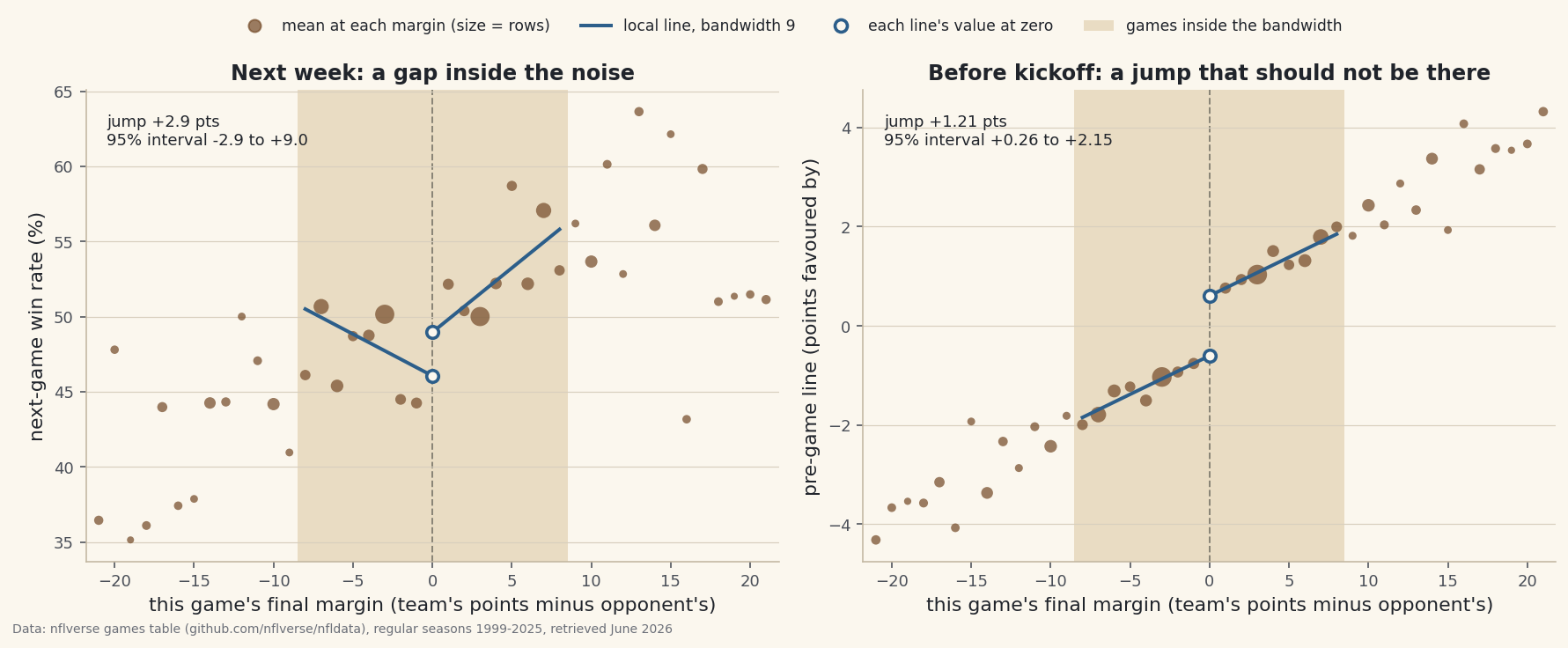
   Regression discontinuity studies lead with the same picture: the outcome averaged at each value of the running variable, a fitted line on each side, and the gap at the cutoff. Draw it twice, for the next-week win rate and for the pre-game line, with the bandwidth shaded so a reader can see which games the lines were allowed to use.

   import matplotlib.pyplot as plt
   
   fig, axes = plt.subplots(1, 2, figsize=(12.4, 5.0))
   panels = ((x_out, y_win, out, "next_win", 100, "next-game win rate (%)"),
             (x_dec, y_line, dec, "line", 1, "pre-game line (points favoured by)"))
   for ax, (x, y, frame, col, scale, label) in zip(axes, panels):
       cells = frame[frame.margin.abs() <= 21].groupby("margin")[col].agg(["size", "mean"])
       ax.axvspan(-(H - 0.5), H - 0.5, color="#E9DCC3", lw=0)     # the bandwidth
       ax.axvline(0, color="grey", ls="--", lw=1)                 # the cutoff
       ax.scatter(cells.index, scale * cells["mean"], s=8 + cells["size"] / 9,
                  color="#7A5230", alpha=0.75)
       for right in (True, False):
           a, b = side_line(x, y, H, right)
           grid = np.linspace(0, H - 1, 50) * (1 if right else -1)
           ax.plot(grid, a + b * grid, color="#2C5E8A", lw=2)
           ax.scatter([0], [a], s=46, facecolor="white", edgecolor="#2C5E8A", zorder=4)
       ax.set_xlabel("this game's final margin")
       ax.set_ylabel(label)
   fig.tight_layout()
   fig.savefig("rd_close_wins.png", dpi=144)

   

   The two panels are the argument at a glance. On the left the lines reach zero 2.9 points apart, while the sixteen cell means inside the window run from 44.24% to 58.70%. On the right the cell means climb the margin in a tight band and the two lines arrive at zero 1.21 points apart. What we set out to measure does not jump; the thing that should never jump does.

Where this breaks

Six limits. The running variable is whole numbers, and lumpy. No game ends at a margin of half a point, so every estimate here extrapolates from one point to zero, and nearly a quarter of decided games land on exactly 3 or 7. The common repair for a discrete running variable, clustering standard errors by its values, is the practice Kolesár and Rothe (2018) show does not protect coverage; our intervals are a plain bootstrap and should be read as approximate. The bandwidth is a football convention, not an optimum. One-score games make a defensible window. Data-driven bandwidths and the robust nonparametric intervals of Calonico, Cattaneo and Titiunik (2014), built to account for the bias a local line carries, could move these numbers, and the six-window sweep is how we show the conclusions do not hang on the choice. The question is narrow. The estimate is the effect of winning rather than losing at a margin of zero; a twenty-point win is not identified by this design at all. The balance failure clouds the causal reading. Narrow winners were slightly better teams, so the next-week jumps are an effect plus a small head start. We have argued that the head start pushes them up, which only strengthens the null, but we have not removed it. One week is one outcome. A W also goes into the standings, and what it is worth to a playoff race is arithmetic this design does not touch. And the line is one market’s closing price, a pre-game summary that already knows the injury report and the weather: the best single measure of strength going in, and still only an estimate of it.

Sources. Games, scores and closing lines: the nflverse games table, June 2026 snapshot, bundled by build/make_nfl_lines_csv.py as nfl_games_lines.csv; the overtime flag from the same snapshot, bundled by build/make_nfl_overtime_csv.py as nfl_games_overtime.csv; attribution to nflverse required. The method: D. L. Thistlethwaite and D. T. Campbell, “Regression-Discontinuity Analysis: An Alternative to the Ex Post Facto Experiment,” Journal of Educational Psychology 51(6), 1960, pp. 309-317, doi:10.1037/h0044319. Practice: G. W. Imbens and T. Lemieux, “Regression Discontinuity Designs: A Guide to Practice,” Journal of Econometrics 142(2), 2008, pp. 615-635, doi:10.1016/j.jeconom.2007.05.001. Close contests as experiments: D. S. Lee, “Randomized Experiments from Non-random Selection in U.S. House Elections,” Journal of Econometrics 142(2), 2008, pp. 675-697, doi:10.1016/j.jeconom.2007.05.004; and the imbalance that complicates them, D. Caughey and J. S. Sekhon, “Elections and the Regression Discontinuity Design: Lessons from Close U.S. House Races, 1942-2008,” Political Analysis 19(4), 2011, pp. 385-408, doi:10.1093/pan/mpr032. The density test: J. McCrary, “Manipulation of the Running Variable in the Regression Discontinuity Design: A Density Test,” Journal of Econometrics 142(2), 2008, pp. 698-714, doi:10.1016/j.jeconom.2007.05.005. Discrete running variables: M. Kolesár and C. Rothe, “Inference in Regression Discontinuity Designs with a Discrete Running Variable,” American Economic Review 108(8), 2018, pp. 2277-2304, doi:10.1257/aer.20160945. Robust intervals: S. Calonico, M. D. Cattaneo and R. Titiunik, “Robust Nonparametric Confidence Intervals for Regression-Discontinuity Designs,” Econometrica 82(6), 2014, pp. 2295-2326, doi:10.3982/ECTA11757. A sports discontinuity that did find a jump: J. Berger and D. Pope, “Can Losing Lead to Winning?” Management Science 57(5), 2011, pp. 817-827, doi:10.1287/mnsc.1110.1328, in which professional basketball teams behind by a point at halftime won more often than teams ahead by one. Every number on this page is recomputed by the tutorial’s script, whose asserts fail rather than print a figure they cannot reproduce.

Troubleshooting