Gaussian Mixtures: EM Finds the Court's Zones

Every shot in an NBA shot log comes with two numbers, where on the floor it was taken, and nothing in those two numbers says “corner three” or “restricted area.” A Gaussian mixture model assumes the points were drawn from a few overlapping bell shapes, and the EM algorithm finds the shapes by alternating two steps simple enough to write in a dozen lines. Run on the coordinates of 24,947 half-court shots from the 2023-24 season, six components that never saw the league’s zone labels agree with them on 85.4% of shots. K-means, given the same six clusters, manages 67.3%, because its clusters are round and the corner three is not: the mixture draws each corner as a strip about half a foot wide, holding all 1,310 left-corner threes and 1,252 of the 1,253 on the right. Then the method shows its weak spot. 704 shots in the file are logged at exactly the middle of the basket, and an eight-component fit pulls one component onto that single point, where the likelihood has no maximum: every tenfold shrink of its spread adds 3,242 to the log-likelihood. With a floor under the spread the fit settles, but the Bayesian information criterion spends a component on that one spot from eight components up and is still asking for more at ten. The likelihood finds the court’s zones, and it rewards a recording habit just as readily.

Bring the k-means tutorial, because a Gaussian mixture is k-means with soft edges and shapes, and the league-wide shot heatmap, which draws the same 25,000 shots this page clusters. Principal component analysis was the course’s last look at data without labels; this one asks a different question of it, which groups the rows fall into rather than which directions they spread along. Everything runs offline from the bundled nba_league_shots.csv, a 25,000-shot random sample of the 2023-24 regular season from the public NBA_Shots_04_25 shot log. No scikit-learn and no scipy: the mixture, the EM loop and k-means are all written out in numpy.

1. The court in feet

   Two columns, LOC_X and LOC_Y, place each shot on the floor. The file does not say where the basket is, so the first job is to find it. If the basket sits at x = 0, y = 5.25 feet, then the distance from that point, rounded down to whole feet, should reproduce the file’s own SHOT_DISTANCE column. The 53 backcourt heaves go, since a half-court model has no use for them, and the league’s zone label, BASIC_ZONE, is kept only to grade the clusters later; the model never sees it.

   import numpy as np
   import pandas as pd
   
   shots = pd.read_csv("nba_league_shots.csv")
   r = np.hypot(shots.LOC_X, shots.LOC_Y - 5.25)            # feet from the middle of the basket
   print(f"{len(shots):,} shots; floor(r) equals SHOT_DISTANCE on {(np.floor(r) == shots.SHOT_DISTANCE).mean():.3%}")
   
   shots = shots[shots.BASIC_ZONE != "Backcourt"].reset_index(drop=True)
   X = shots[["LOC_X", "LOC_Y"]].to_numpy(float)
   dist = np.hypot(X[:, 0], X[:, 1] - 5.25)
   print(f"{len(shots):,} half-court shots, |x| at most {np.abs(X[:, 0]).max()} ft")
   for zone, n in shots.BASIC_ZONE.value_counts().items():
       print(f"  {zone:22s} {n:5,d}")
   
   three = (shots.SHOT_TYPE == "3PT Field Goal").to_numpy()
   low = X[:, 1] < 14                                       # the straight part of the line
   print(f"threes below y = 14: none closer than {np.abs(X[three & low, 0]).min()} ft to the middle line;"
         f" threes above: none closer than {dist[three & ~low].min():.2f} ft to the basket")
   print("threes the zone column calls Mid-Range:", int((three & (shots.BASIC_ZONE == "Mid-Range")).sum()))
   
   spots = shots.groupby(["LOC_X", "LOC_Y"]).size().sort_values(ascending=False)
   at_rim = (shots.LOC_X == 0) & (shots.LOC_Y == 5.25)
   print(f"busiest spot: x = 0, y = 5.25, {spots.iloc[0]} shots ({at_rim.mean():.2%});"
         f" next busiest: {spots.iloc[1]}")

   The basket is at (0, 5.25); 704 shots sit exactly on it

   25,000 shots; floor(r) equals SHOT_DISTANCE on 99.892%
   24,947 half-court shots, |x| at most 25.0 ft
     Restricted Area        7,379
     Above the Break 3      7,255
     In The Paint (Non-RA)  4,971
     Mid-Range              2,779
     Left Corner 3          1,310
     Right Corner 3         1,253
   threes below y = 14: none closer than 21.9 ft to the middle line; threes above: none closer than 23.77 ft to the basket
   threes the zone column calls Mid-Range: 4
   busiest spot: x = 0, y = 5.25, 704 shots (2.82%); next busiest: 22

   The distance check holds on 99.892% of the 25,000 rows, 24,973 of them, and each of the 27 exceptions sits exactly on a whole number of feet, where floating-point arithmetic lands a hair below it, so the coordinates are in feet with the middle of the basket at (0, 5.25). The rulebook fixes the rest of the geometry. Rule No. 1 puts the three-point line on “parallel lines 3′ from the sidelines, extending from the baseline and an arc of 23′9″ from the middle of the basket,” and the file agrees: no x is further than 25.0 feet from the middle, so the sidelines are at ±25 and the straight part of the line at ±22; no three below y = 14 is closer than 21.9 feet to the middle line, and none above it closer than 23.77 feet to the basket, the 23.75-foot arc to the file’s tenth-of-a-foot precision. Four threes carry the zone label Mid-Range, a small reminder that the labels the clusters will be graded against are themselves a separate recording.

   The last line is the one that matters later. The busiest single coordinate in the file is the basket itself: 704 shots, 2.82% of the half court, are logged at exactly x = 0, y = 5.25, all of them two-pointers in the restricted area with a recorded distance of zero. The next busiest coordinate holds 22. Real shots near the rim are spread over a few feet; these 704 share one point to the hundredth of a foot. The file cannot say why, and nothing below depends on knowing, but a model that measures how tightly points cluster is going to notice.

2. EM on paper: one dimension, two components

   Start with one number per shot, its distance from the basket, and two bell curves: one for shots near the rim and one for shots from range. A mixture of two normal distributions has five unknowns, two means, two standard deviations and the share of shots in the first component (the second share is what is left). If every shot came labelled with its component, each curve could be fitted by an ordinary mean and standard deviation. If the curves were known, Bayes’ rule would give each shot’s probability of belonging to each one. EM does both in turn. The E-step computes those probabilities, called responsibilities, from the current curves. The M-step refits each curve as a weighted mean and standard deviation, every shot counted in proportion to its responsibility. Dempster, Laird and Rubin (1977) gave the algorithm its name and the proof that matters in practice: no round can lower the likelihood.

   def normal_pdf(x, mean, sd):
       return np.exp(-0.5 * ((x - mean) / sd) ** 2) / (sd * np.sqrt(2 * np.pi))
   
   def em_1d(x, w, mean, sd, tol=1e-8, max_iter=1000):
       history = []
       for it in range(max_iter):
           dens = w * normal_pdf(x[:, None], mean, sd)      # E-step: weight x density...
           total = dens.sum(axis=1)
           history.append(np.log(total).sum())            # (the log-likelihood so far)
           resp = dens / total[:, None]                    # ...as each component's share
           nk = resp.sum(axis=0)                           # M-step: shots per component,
           w = nk / len(x)                                 # its weight,
           mean = (resp * x[:, None]).sum(axis=0) / nk     # its mean
           sd = np.sqrt((resp * (x[:, None] - mean) ** 2).sum(axis=0) / nk)   # and its spread
           if it and history[-1] - history[-2] < tol:
               break
       return w, mean, sd, history
   
   w1, m1, s1, hist = em_1d(dist, np.array([0.5, 0.5]), np.array([5.0, 25.0]), np.array([5.0, 5.0]))
   print(f"{len(hist)} rounds; log-likelihood {hist[0]:,.1f} -> {hist[1]:,.1f} -> {hist[2]:,.1f}"
         f" ... {hist[-1]:,.2f}; it never fell: {bool(np.all(np.diff(hist) >= 0))}")
   print(f"near: weight {w1[0]:.4f}, mean {m1[0]:.3f} ft, sd {s1[0]:.3f}")
   print(f"far:  weight {w1[1]:.4f}, mean {m1[1]:.3f} ft, sd {s1[1]:.3f}")
   
   parts = w1 * normal_pdf(22.0, m1, s1)                   # one shot from 22 feet
   print(f"22 ft: near {parts[0]:.6f}, far {parts[1]:.6f}, far share {parts[1] / parts.sum():.4f}")
   
   grid = np.arange(0, 80, 0.001)
   lead = np.sign(w1[1] * normal_pdf(grid, m1[1], s1[1]) - w1[0] * normal_pdf(grid, m1[0], s1[0]))
   flips = grid[1:][np.diff(lead) != 0]
   inside = (dist > flips[0]) & (dist < flips[1])
   print(f"the far component wins from {flips[0]:.2f} to {flips[1]:.2f} ft:"
         f" {inside.sum():,} shots, {three[inside].mean():.1%} of them threes")
   print(f"shots beyond {flips[1]:.2f} ft, handed back to the near component: {(dist > flips[1]).sum()}")

   39 rounds; the far component wins from 19.86 ft and gives the heaves back

   39 rounds; log-likelihood -86,645.0 -> -84,802.2 -> -84,625.8 ... -83,799.33; it never fell: True
   near: weight 0.5924, mean 6.065 ft, sd 5.444
   far:  weight 0.4076, mean 25.361 ft, sd 1.984
   22 ft: near 0.000599, far 0.019526, far share 0.9703
   the far component wins from 19.86 to 36.78 ft: 10,179 shots, 96.3% of them threes
   shots beyond 36.78 ft, handed back to the near component: 19

   From a deliberately rough start, means of 5 and 25 feet and a spread of 5 for both, the log-likelihood rises in every one of the 39 rounds, from −86,645.0 to −83,799.33, the monotone climb the 1977 paper proved. The fit settles on a near component holding 59.24% of shots around 6.065 feet with a wide spread of 5.444, and a far component holding 40.76% at 25.361 feet with a spread of only 1.984. That narrow far curve is the three-point line: shooters stand just behind it, so distances from range pile up in a tight band.

   The worked example shows one E-step by hand. A shot from 22 feet is 2.9271 near-component standard deviations above that mean, (22 − 6.065)/5.444, so its density there is e^−4.2839/(5.444 × √(2π)) = 0.01379/13.6461 = 0.0010105, and weighted by 0.5924 that is 0.000599. Under the far component it is 1.6941 standard deviations below the mean: e^−1.4349/(1.984 × √(2π)) = 0.23814/4.9732 = 0.047885, weighted by 0.4076, 0.019518. The far component’s responsibility is 0.019518/(0.019518 + 0.000599) = 0.9702 with these rounded numbers, 0.9703 with the full ones. Every shot gets the same treatment, and the M-step averages over all of them.

   The boundary between the components, where the two weighted curves cross, falls at 19.86 feet, two feet inside the corner line and four inside the arc. A mixture does not draw lines; it draws curves, and where they cross depends on their weights and spreads as much as on their means. Between 19.86 and 36.78 feet the far component wins, a range holding 10,179 shots of which 96.3% are threes. Past 36.78 feet the near component wins again: its wide curve falls away more slowly than the narrow far one, so the 19 half-court shots from beyond 36.78 feet, the longest heaves, are assigned to the component centred six feet from the rim. That is not a bug in the code. It is what two normal curves with unequal spreads imply, and it is the first sign that a mixture describes the shape of the data, not its meaning.

3. Two dimensions: full covariances and ten starts

   In two dimensions each component needs a centre, a 2 × 2 covariance matrix (two spreads and the correlation between x and y, which lets an ellipse tilt) and a weight: six numbers each, less one for the weights summing to one. The E-step and M-step are the same as before with vectors in place of numbers. Two practical changes come with them. Densities of points far from a component underflow to zero in floating point, so the E-step works with logarithms and the log-sum-exp trick: subtract each row’s largest log term before exponentiating, then add it back. And EM only climbs to the nearest peak of the likelihood, so the fit is run from ten different random starts and the best kept, the same habit k-means needs.

   def log_normal_2d(X, mean, cov):
       """log density of every shot under every component: an (n, k) table."""
       a, b, c = cov[:, 0, 0], cov[:, 0, 1], cov[:, 1, 1]
       det = a * c - b * b
       dx = X[:, None, 0] - mean[None, :, 0]
       dy = X[:, None, 1] - mean[None, :, 1]
       q = (c * dx * dx - 2 * b * dx * dy + a * dy * dy) / det   # the 2 x 2 inverse, written out
       return -0.5 * q - np.log(2 * np.pi) - 0.5 * np.log(det)
   
   def gmm(X, k, seed, floor=0.0, tol=1e-3, max_iter=1000):
       rng = np.random.default_rng(seed)
       mean = X[rng.choice(len(X), k, replace=False)]        # start: k random shots as centres
       cov = np.repeat(np.cov(X.T, bias=True)[None], k, axis=0)
       w = np.full(k, 1 / k)
       history = []
       for it in range(1, max_iter + 1):
           L = np.log(w) + log_normal_2d(X, mean, cov)
           top = L.max(axis=1)
           lse = top + np.log(np.exp(L - top[:, None]).sum(axis=1))   # log-sum-exp, no underflow
           history.append(lse.sum())
           resp = np.exp(L - lse[:, None])                    # E-step
           nk = resp.sum(axis=0)                              # M-step
           d = X[:, None, :] - (resp.T @ X / nk[:, None])[None]
           new_cov = np.einsum("nk,nki,nkj->kij", resp, d, d) / nk[:, None, None] + floor * np.eye(2)
           det = new_cov[:, 0, 0] * new_cov[:, 1, 1] - new_cov[:, 0, 1] ** 2
           if det.min() < 1e-9:                               # a component has shrunk onto a point
               return dict(w=w, mean=mean, cov=cov, resp=resp, ll=history[-1], it=it,
                           history=history, collapsed=True)
           w, mean, cov = nk / len(X), resp.T @ X / nk[:, None], new_cov
           if it > 1 and history[-1] - history[-2] < tol:
               break
       return dict(w=w, mean=mean, cov=cov, resp=resp, ll=history[-1], it=it,
                   history=history, collapsed=False)
   
   fits = [gmm(X, 6, seed) for seed in range(10)]
   lls = np.array([f["ll"] for f in fits])
   print("ten starts, final log-likelihoods:", ", ".join(f"{v:,.1f}" for v in sorted(lls)))
   best = fits[int(lls.argmax())]
   order = np.lexsort((best["mean"][:, 0], best["mean"][:, 1]))   # one fixed order for the labels
   w6, mean6, cov6 = best["w"][order], best["mean"][order], best["cov"][order]
   label = best["resp"][:, order].argmax(axis=1)
   
   table = pd.crosstab(label, shots.BASIC_ZONE)
   print(" comp  weight   centre (x, y)   sd x   sd y   corr  largest zone            share  makes")
   for j in range(6):
       sx, sy = np.sqrt(cov6[j, 0, 0]), np.sqrt(cov6[j, 1, 1])
       top = table.loc[j].idxmax()
       print(f"  {j + 1}   {w6[j]:.3f}  ({mean6[j, 0]:6.2f},{mean6[j, 1]:6.2f})  {sx:5.2f}  {sy:5.2f}"
             f"  {cov6[j, 0, 1] / (sx * sy):+.2f}  {top:22s}  {table.loc[j, top] / table.loc[j].sum():.3f}"
             f"  {shots.SHOT_MADE[label == j].mean():.3f}")
   purity = table.max(axis=1).sum() / len(shots)
   print(f"shots in their component's largest zone: {purity:.1%}")
   worst = fits[int(lls.argmin())]
   print("corner strips (sd x under 0.6 ft) in the best fit:", int((np.sqrt(cov6[:, 0, 0]) < 0.6).sum()),
         "; in the lowest:", int((np.sqrt(worst["cov"][:, 0, 0]) < 0.6).sum()))

   Six components; 85.4% of shots land in their component's largest zone

   ten starts, final log-likelihoods: -164,167.4, -164,167.4, -159,642.3, -159,642.3, -159,642.3, -159,642.3, -159,642.3, -159,642.3, -159,642.3, -159,642.3
    comp  weight   centre (x, y)   sd x   sd y   corr  largest zone            share  makes
     1   0.303  ( -0.11,  6.54)   1.70   1.16  -0.06  Restricted Area         0.930  0.643
     2   0.056  ( 23.11,  7.65)   0.51   3.33  -0.10  Left Corner 3           0.930  0.387
     3   0.057  (-23.04,  8.81)   0.55   3.92  +0.23  Right Corner 3          0.870  0.384
     4   0.301  ( -0.27, 13.03)   7.50   5.05  -0.01  In The Paint (Non-RA)   0.625  0.430
     5   0.131  ( 13.74, 26.65)   5.43   4.04  -0.86  Above the Break 3       0.984  0.360
     6   0.151  (-10.50, 28.04)   7.10   3.67  +0.81  Above the Break 3       0.975  0.360
   shots in their component's largest zone: 85.4%
   corner strips (sd x under 0.6 ft) in the best fit: 2 ; in the lowest: 0

   Eight of the ten starts reach the same peak, a log-likelihood of −159,642.3; two stop at −164,167.4, a different and worse answer, not a rounding difference. The lower one has no corner strips at all. It covers the whole baseline, both corners and the space between, with one flat component whose standard deviations are 17.6 feet across the floor and 1.9 feet deep. A single run of EM would have returned either with equal confidence; only the comparison says which is better. Component numbers are arbitrary as well (any permutation of the six is the same fit, which is called label switching), so the code sorts them by their centres before printing.

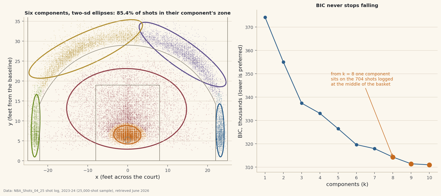
   Read down the table and the court appears. Component 1 holds 30.3% of shots in a tight ellipse around the rim, with spreads of 1.70 and 1.16 feet; 93.0% of its shots are in the restricted area and 64.3% of them went in. Components 2 and 3 are the corners: centres 23.11 and 23.04 feet from the middle line, spreads across the floor of only 0.51 and 0.55 feet against 3.33 and 3.92 along it. They are the shape of the space between the line at 22 feet and the sideline at 25. The left strip holds all 1,310 left-corner threes, the right 1,252 of the 1,253 right-corner ones. Components 5 and 6 split the arc above the break into its two sides, each a long ellipse with a correlation of −0.86 or +0.81 between x and y because the arc is curved; 98.4% and 97.5% of their shots are above-the-break threes. Component 4 is everything else, a broad ellipse with spreads of 7.50 and 5.05 feet over the paint and the mid-range; it holds 94.4% of the file’s mid-range shots, so six components buy no separate mid-range zone. Graded against the league’s six labels, 85.4% of shots fall in their component’s largest zone. A mixture of six components cannot score 100% against six zones that include two with no shape of their own, but most of the map is there.

4. The likelihood that runs to infinity

   Ask for eight components and run the same loop from start 0. The loop above has a guard for this: it stops if any component’s covariance determinant, the area of its ellipse squared up to a constant, falls below 10⁻⁹. The output shows why the guard is needed.

   bad = gmm(X, 8, seed=0)
   h = np.array(bad["history"])
   print(f"8 components, start 0: collapsed = {bad['collapsed']} at round {bad['it']}")
   print("last rounds' log-likelihood:", ", ".join(f"{v:,.0f}" for v in h[-6:]))
   sds = np.sqrt(bad["cov"][:, [0, 1], [0, 1]])
   j = int(np.argmin(sds.prod(axis=1)))
   print(f"component {j}: weight x shots = {bad['w'][j] * len(X):.1f}, centre ({bad['mean'][j, 0]:.4f},"
         f" {bad['mean'][j, 1]:.4f}), sd ({sds[j, 0]:.2e}, {sds[j, 1]:.2e}) ft")
   owned = bad["resp"][:, j] > 0.5
   print(f"shots it owns: {owned.sum()}, {int(at_rim[owned].sum())} of them at the basket spot;"
         f" the nearest owned shot that is not: {np.hypot(*(X[owned & ~at_rim] - [0, 5.25]).T).min():.2f} ft away")
   print(f"every tenfold shrink of both sds adds 704 x 2 ln 10 = {704 * 2 * np.log(10):,.1f}")
   
   ok = gmm(X, 8, seed=0, floor=0.01)                         # a floor: no sd below 0.1 ft
   sds = np.sqrt(ok["cov"][:, [0, 1], [0, 1]])
   j = int(np.argmin(sds.prod(axis=1)))
   print(f"with the floor: collapsed = {ok['collapsed']}, log-likelihood {ok['ll']:,.1f};"
         f" tightest component weight x shots = {ok['w'][j] * len(X):.1f},"
         f" sd ({sds[j, 0]:.3f}, {sds[j, 1]:.3f})")

   One component shrinks onto the 704 basket-spot shots; a floor stops it

   8 components, start 0: collapsed = True at round 189
   last rounds' log-likelihood: -157,462, -157,197, -156,919, -156,551, -155,941, -154,691
   component 1: weight x shots = 738.8, centre (0.0004, 5.2520), sd (1.23e-02, 2.77e-02) ft
   shots it owns: 725, 704 of them at the basket spot; the nearest owned shot that is not: 0.10 ft away
   every tenfold shrink of both sds adds 704 x 2 ln 10 = 3,242.0
   with the floor: collapsed = False, log-likelihood -156,918.6; tightest component weight x shots = 824.2, sd (0.115, 0.120)

   At round 189 the guard fires. Over the last five rounds the log-likelihood jumped from −157,462 to −154,691, by far the fastest rise of the fit, and none of it came from describing the court better. One component has moved to (0.0004, 5.2520) with standard deviations of 0.012 and 0.028 feet, and it owns 725 shots, 704 of them the identical basket-spot coordinates and the rest within a tenth of a foot. One more M-step would have pushed its determinant below the guard’s 10⁻⁹, on the way to zero and an infinite density.

   The arithmetic is the whole explanation. A component with weight w sitting exactly on 704 identical points gives each of them a log density of log w − log(2π) − log(σ_xσ_y), and nothing else in the likelihood stops σ from shrinking. Divide both standard deviations by ten and each of the 704 points gains 2 ln 10, 3,242.0 in total, again and again without end. The likelihood of a Gaussian mixture has no maximum whenever a component can sit on one point, so what EM returns is a local peak, never a global maximum, which does not exist; Redner and Walker (1984) review maximum likelihood for mixtures and the EM algorithm at length. Usually the singularity needs bad luck, a component wandering onto a single point. Here the data offers one.

   The standard repair is a floor: add a small constant to the diagonal of every covariance at every M-step, so no spread can fall below it. The floor here is 0.01 square feet, a standard deviation of 0.1 feet, the precision the file records. With it the same start finishes cleanly at −156,918.6, and the tightest component is still on the basket spot, holding 824.2 shots’ worth of weight with spreads of 0.115 and 0.120 feet, just above the floor. The floor turned an infinite reward into a large finite one. It did not stop the model wanting the spot.

5. How many components?

   More components always fit at least as well, so the number has to be chosen by something that charges for them. Schwarz (1978) proposed the Bayesian information criterion, BIC = −2 × log-likelihood + p × ln n, where p is the number of free parameters (6k − 1 here) and n the number of shots; lower is better. For mixtures used as clustering models more broadly, see Fraley and Raftery (2002). The sweep below fits one to ten components with the floor in place, four starts each.

   def bic(fit, k, n):
       return -2 * fit["ll"] + (6 * k - 1) * np.log(n)        # 6k - 1 free numbers
   
   sweep = []
   for k in range(1, 11):
       runs = [gmm(X, k, seed, floor=0.01) for seed in range(4)]
       top = max(runs, key=lambda f: f["ll"])
       sds = np.sqrt(top["cov"][:, [0, 1], [0, 1]]).prod(axis=1)
       spot = bool((sds < 0.02).any())                        # a component sitting on one spot?
       sweep.append((k, top["ll"], bic(top, k, len(X)), spot))
       print(f"k = {k:2d}  log-likelihood {top['ll']:12,.1f}  BIC {sweep[-1][2]:11,.1f}"
             f"  on the basket spot: {'yes' if spot else 'no'}")
   drops = np.diff([s[2] for s in sweep])
   print(f"BIC falls at every step; smallest fall {-drops.max():,.1f} (k = 9 to 10)")

   BIC falls at every k; from eight up one component sits on the basket spot

   k =  1  log-likelihood   -187,056.9  BIC   374,164.4  on the basket spot: no
   k =  2  log-likelihood   -177,443.8  BIC   354,998.9  on the basket spot: no
   k =  3  log-likelihood   -168,613.1  BIC   337,398.4  on the basket spot: no
   k =  4  log-likelihood   -166,400.2  BIC   333,033.2  on the basket spot: no
   k =  5  log-likelihood   -163,084.9  BIC   326,463.3  on the basket spot: no
   k =  6  log-likelihood   -159,643.8  BIC   319,641.9  on the basket spot: no
   k =  7  log-likelihood   -158,748.3  BIC   317,911.8  on the basket spot: no
   k =  8  log-likelihood   -156,918.6  BIC   314,313.1  on the basket spot: yes
   k =  9  log-likelihood   -155,446.2  BIC   311,428.9  on the basket spot: yes
   k = 10  log-likelihood   -155,200.5  BIC   310,998.3  on the basket spot: yes
   BIC falls at every step; smallest fall 430.6 (k = 9 to 10)

   BIC never turns. It falls from 374,164.4 at one component to 310,998.3 at ten, and even the smallest step, nine to ten, saves 430.6, far more than the ln n × 6 = 60.7 each extra component costs. From eight components on, the best fit of the four starts always spends one component on the 704 basket-spot shots, and that one move is worth a fall of 3,598.7 between seven and eight. BIC is doing its job. Its job is to measure how well a set of ellipses reproduces the density of the points, and with 24,947 points it can afford to reproduce every lump: the spike at the basket, the tight band behind the arc, the pile of layups just off the rim. It does not know what a zone is.

   So the honest answer to “how many components?” depends on the question. As a density model, more than ten. As a map of the court, six already returns the restricted area, the two corners and the two sides of the arc, and the components that follow split lumps rather than finding new places to shoot from. Neither the likelihood nor BIC can make that call, because both reward the 704 identical coordinates exactly as they reward a real zone.

6. Soft edges, and what k-means misses

   A mixture gives every shot a probability for every component instead of one label. That is most of what it adds to k-means, which assigns each point to its nearest centre and implicitly assumes every cluster is a circle of the same size. The comparison is k-means run on the same coordinates with the same six clusters and ten starts.

   resp6 = best["resp"][:, order]
   sure = resp6.max(axis=1)
   print(f"shots at least 99% in one component: {(sure >= 0.99).mean():.1%};"
         f" under 90%: {(sure < 0.9).mean():.1%}; under 60%: {(sure < 0.6).sum():,}")
   split = sure < 0.6
   print("where the split shots are:", shots.BASIC_ZONE[split].value_counts().head(3).to_dict())
   
   def kmeans(X, k, seed, max_iter=500):
       rng = np.random.default_rng(seed)
       c = X[rng.choice(len(X), k, replace=False)]
       for _ in range(max_iter):
           lab = ((X[:, None] - c[None]) ** 2).sum(axis=2).argmin(axis=1)
           new = np.array([X[lab == j].mean(axis=0) for j in range(k)])
           if np.allclose(new, c):
               break
           c = new
       return lab, c, ((X - c[lab]) ** 2).sum()
   
   lab_km, c_km, _ = min((kmeans(X, 6, s) for s in range(10)), key=lambda t: t[2])
   table_km = pd.crosstab(lab_km, shots.BASIC_ZONE)
   print(f"k-means, six clusters, ten starts: {table_km.max(axis=1).sum() / len(shots):.1%} in their largest zone")
   for zone in ("Left Corner 3", "Right Corner 3"):
       jk = table_km[zone].idxmax()
       print(f"  the k-means cluster holding the {zone}s: {table_km.loc[jk].sum():,} shots,"
             f" {table_km.loc[jk, zone] / table_km.loc[jk].sum():.1%} of them corner threes")

   Half the shots are 99% certain; k-means scores 67.3% to the mixture's 85.4%

   shots at least 99% in one component: 50.5%; under 90%: 14.1%; under 60%: 589
   where the split shots are: {'In The Paint (Non-RA)': 365, 'Above the Break 3': 169, 'Mid-Range': 52}
   k-means, six clusters, ten starts: 67.3% in their largest zone
     the k-means cluster holding the Left Corner 3s: 1,873 shots, 69.9% of them corner threes
     the k-means cluster holding the Right Corner 3s: 1,894 shots, 66.2% of them corner threes

   Half the shots, 50.5%, are at least 99% in one component; 14.1% are under 90%, and 589 are under 60%, genuinely split. Most of the split shots are in the paint outside the restricted area (365) or above the break (169), where the rim ellipse meets the broad paint one and where the two arc components meet at the top of the key. A hard label would hide that those shots sit on a boundary; the responsibilities say so directly.

   K-means puts 67.3% of shots in their cluster’s largest zone, 18.1 points below the mixture. The difference is in the corners. Each k-means corner cluster does contain every corner three on its side, but it also takes the baseline mid-range shots next to them: the left one holds 1,873 shots of which 69.9% are corner threes, the right 1,894 with 66.2%. A circle cannot be half a foot wide and seven feet long. The mixture’s covariance can, which is why its corner strips are 93.0% and 87.0% corner threes. The same freedom produced the collapse in step four, since a covariance that can be as thin as the data wants can also be thinner than any real zone.

7. Draw the fit

   Two panels carry the argument: the six components on the court, each drawn as the ellipse two standard deviations from its centre over the shots it claims, and the BIC sweep with the basket-spot fits marked.

   import matplotlib.pyplot as plt
   from matplotlib.patches import Arc, Ellipse
   
   def court(ax):
       """Half-court lines in the file's feet: basket at (0, 5.25), sidelines at x = +-25."""
       kw = dict(color="#8A8577", lw=1)
       ax.plot([-25, 25, 25, -25, -25], [0, 0, 47, 47, 0], **kw)
       ax.plot([-22, -22], [0, 5.25 + np.sqrt(23.75 ** 2 - 22 ** 2)], **kw)
       ax.plot([22, 22], [0, 5.25 + np.sqrt(23.75 ** 2 - 22 ** 2)], **kw)
       t = np.degrees(np.arctan2(np.sqrt(23.75 ** 2 - 22 ** 2), 22))
       ax.add_patch(Arc((0, 5.25), 47.5, 47.5, theta1=t, theta2=180 - t, **kw))
       ax.plot([-8, -8, 8, 8], [0, 19, 19, 0], **kw)
       ax.add_patch(Arc((0, 5.25), 1.5, 1.5, **kw))
   
   COLORS = ["#C56A1E", "#2C5E8A", "#6B8E23", "#8E3B46", "#5B4B8A", "#B08D2E"]
   fig, (ax1, ax2) = plt.subplots(1, 2, figsize=(12.6, 5.6), gridspec_kw={"width_ratios": [1.15, 1]})
   for j in range(6):
       pts = X[label == j]
       ax1.scatter(pts[:, 0], pts[:, 1], s=2, color=COLORS[j], alpha=0.25, linewidths=0)
   for j in range(6):
       vals, vecs = np.linalg.eigh(cov6[j])
       ang = np.degrees(np.arctan2(vecs[1, 1], vecs[0, 1]))
       ax1.add_patch(Ellipse(mean6[j], 4 * np.sqrt(vals[1]), 4 * np.sqrt(vals[0]), angle=ang,
                             fill=False, color=COLORS[j], lw=2))
   court(ax1)
   ax1.set_xlim(-26, 26)
   ax1.set_ylim(-1, 36)
   ax1.set_aspect("equal")
   ax1.set_xlabel("x (feet across the court)")
   ax1.set_ylabel("y (feet from the baseline)")
   ax1.set_title(f"Six components, two-sd ellipses: {purity:.1%} of shots in their component's zone",
                 fontsize=10)
   
   ks = [s[0] for s in sweep]
   ax2.plot(ks, [s[2] / 1000 for s in sweep], marker="o", color="#2C5E8A")
   for k, _ll, b, spot in sweep:
       if spot:
           ax2.plot(k, b / 1000, marker="o", color="#C56A1E", ms=9)
   ax2.annotate("from k = 8 one component\nsits on the 704 shots logged\nat the middle of the basket",
                xy=(8, sweep[7][2] / 1000), xytext=(4.6, 345), fontsize=9, color="#C56A1E",
                arrowprops=dict(arrowstyle="->", color="#C56A1E"))
   ax2.set_xticks(ks)
   ax2.set_xlabel("components (k)")
   ax2.set_ylabel("BIC, thousands (lower is preferred)")
   ax2.set_title("BIC never stops falling", fontsize=10)
   fig.tight_layout()
   fig.savefig("gmm_court_zones.png", dpi=144)

   

   The left panel is the map: the corner strips run up the sidelines between the line and the edge of the court, the arc ellipses lean with the curve, and the broad paint ellipse swallows the mid-range. In this file’s coordinates positive x is the side the zone column calls left. The right panel is the warning: the curve flattens but never turns, and the orange points, where a component sits on the basket spot, are among its best scores.

Where this breaks

Six limits. The likelihood rewards repeated points. Any coordinate recorded many times, by a default, a rounding rule or a tracking habit, can capture a component, and with no floor the likelihood has no maximum at all; a floor makes the fit finite without making the component meaningful. Look at the busiest values in a dataset before fitting a mixture to it. Normal shapes are an assumption. The three-point line is a hard edge and the sideline another, and a bell curve can only approximate a strip with walls, which is why BIC keeps adding components to patch the shapes. EM finds a local peak. Two of ten starts here stopped at a worse answer with no corner strips; more components mean more peaks, so use several starts and keep the best, and still treat the result as the best one found, not the best one possible. BIC chooses for density, not meaning. With tens of thousands of points it will keep asking for components long after they stop matching anything a coach would name; choose k for the question, and say how it was chosen. The grading labels are another recording. The 85.4% compares one model with the league’s zone column, which includes four threes labelled mid-range and two zones, mid-range and the paint, that have no natural edge between them. And one season, sampled. These are 25,000 of the 2023-24 season’s shots drawn at random, all teams pooled; a team, a player or another season would give different components, and the 704 basket-spot shots are a property of this file, whose cause it does not record.

Sources. Shots: the public NBA_Shots_04_25 shot log (github.com/DomSamangy/NBA_Shots_04_25), 2023-24 season, a 25,000-row random sample (random_state=42) bundled by build/make_nba_samples.py as nba_league_shots.csv. Court dimensions: NBA Official Rules, Rule No. 1, Section I, read 11 October 2026. Mixtures: K. Pearson, “Contributions to the Mathematical Theory of Evolution,” Philosophical Transactions of the Royal Society of London A 185, 1894, pp. 71-110, doi:10.1098/rsta.1894.0003, which set out “to discuss the dissection of abnormal frequency-curves into normal curves” and doubted the general case “could ever be applied in practice to any numerical case”; N. E. Day, “Estimating the Components of a Mixture of Normal Distributions,” Biometrika 56(3), 1969, pp. 463-474, doi:10.1093/biomet/56.3.463. EM: A. P. Dempster, N. M. Laird and D. B. Rubin, “Maximum Likelihood from Incomplete Data via the EM Algorithm,” Journal of the Royal Statistical Society B 39(1), 1977, pp. 1-22, doi:10.1111/j.2517-6161.1977.tb01600.x; C. F. J. Wu, “On the Convergence Properties of the EM Algorithm,” Annals of Statistics 11(1), 1983, doi:10.1214/aos/1176346060; R. A. Redner and H. F. Walker, “Mixture Densities, Maximum Likelihood and the EM Algorithm,” SIAM Review 26(2), 1984, pp. 195-239, doi:10.1137/1026034. Model size: G. Schwarz, “Estimating the Dimension of a Model,” Annals of Statistics 6(2), 1978, doi:10.1214/aos/1176344136; C. Fraley and A. E. Raftery, “Model-Based Clustering, Discriminant Analysis, and Density Estimation,” Journal of the American Statistical Association 97(458), 2002, pp. 611-631, doi:10.1198/016214502760047131. Every number on this page is recomputed by the tutorial’s script, whose asserts fail rather than print a figure they cannot reproduce.

Troubleshooting