Random Forests: A Column of Noise Ranks Third

The decision-tree tutorial ends with a promise: grow many trees on resampled games, let each split look at only a few columns, let the trees vote, and the crowd should beat the single tree. Then rank the columns by how much impurity each one removed. This tutorial keeps both halves of the promise, in numpy, on the same NBA home-win problem and the same 308 held-out games, and the second half goes wrong in a way worth seeing. Four columns join the two net ratings: each side’s days of rest, read from the schedule, and two planted columns that know nothing about basketball, a random number and a coin flip drawn for every game. The voting works: 500 trees that average 59.4% on the held-out games one at a time reach 65.6% together. The ranking does not. Mean decrease in impurity, the score the forest collects as it grows, puts the column of random numbers third of six, at 25.6% of the total against 26.8% for the away team’s net rating and about four times either rest column, and the trees split on it 28,082 times, more than on any real column. Breiman’s out-of-bag shuffle test, which scrambles one column on the games each tree never saw, scores the same column at −0.04 points, which is zero. A forest’s own importance score measures how often a column was handy for carving up the training games, and a column with 923 different values is always handy.

Bring the decision tree, whose Gini split this page reuses and whose challenge it answers, and the bootstrap tutorial, because every tree here grows on a bootstrap resample. The permutation test is the idea behind the shuffle score, and the rest-days study computed rest the same way from the same schedule. Everything runs offline from the bundled nba_ratings.csv and nba_home_results.csv. No scikit-learn and no scipy: the split search, the trees, the voting and both importance scores are written out in numpy.

1. Six columns, two of them planted

   The target is the decision tree’s: did the home team win? The first two columns are its two features, each team’s 2023-24 net rating, which makes this a teaching problem rather than a forecast, since a full-season rating already knows how the season went. The next two come from the dates alone: the days off each side had before the game, zero for the second night of a back-to-back, capped at three, with each team’s first game counted as rested. The last two are planted. noise is a random number between 0 and 1 and coin a random 0 or 1, drawn with a fixed seed and unrelated to anything in the file. Any importance score worth trusting has to put both of them at the bottom. The split is the decision tree’s exactly, the same seed and the same 75/25 cut, so every accuracy below is measured on the same 308 games.

   import numpy as np
   import pandas as pd
   
   ratings = pd.read_csv("nba_ratings.csv")
   nrtg = dict(zip(ratings["Team"], ratings["NRtg"]))
   g = pd.read_csv("nba_home_results.csv", parse_dates=["date"])
   g["home_win"] = (g["home_pts"] > g["away_pts"]).astype(int)
   g["home_nrtg"] = g["home_team"].map(nrtg)
   g["away_nrtg"] = g["away_team"].map(nrtg)
   
   # days off before each game, from the schedule alone (0 = the second night of a back-to-back)
   side = pd.concat([pd.DataFrame({"game": g.index, "side": "home", "team": g.home_team, "date": g.date}),
                     pd.DataFrame({"game": g.index, "side": "away", "team": g.away_team, "date": g.date})])
   side = side.sort_values(["team", "date"])
   side["rest"] = side.groupby("team")["date"].diff().dt.days - 1
   openers = int(side["rest"].isna().sum())
   side["rest"] = side["rest"].fillna(3).clip(upper=3)        # a season opener counts as rested; 3 means 3 or more
   rest = side.pivot(index="game", columns="side", values="rest")
   g["home_rest"], g["away_rest"] = rest["home"], rest["away"]
   
   # two planted columns that carry no information about the game at all
   noise_rng = np.random.default_rng(101)
   g["noise"] = noise_rng.random(len(g))                      # a random number between 0 and 1
   g["coin"] = noise_rng.integers(0, 2, len(g))               # a random 0 or 1
   
   FEATURES = ["home_nrtg", "away_nrtg", "home_rest", "away_rest", "noise", "coin"]
   X = g[FEATURES].to_numpy(float)
   y = g["home_win"].to_numpy()
   
   idx = np.random.default_rng(76).permutation(len(X))        # the decision-tree tutorial's split, exactly
   cut = int(0.75 * len(X))
   tr, te = idx[:cut], idx[cut:]
   
   print(f"{len(g):,} games: {len(tr)} to train on, {len(te)} held out "
         f"(home teams won {y[te].mean():.1%} of the held-out games)")
   print(f"rest, days off before a game, over {len(side):,} team-games ({openers} season openers counted as 3):")
   for d, n in side["rest"].value_counts().sort_index().items():
       print(f"  {int(d)}{'+' if d == 3 else ' '}  {n:5,d}")
   print("distinct values in the training games:")
   for j, f in enumerate(FEATURES):
       print(f"  {f:10s} {len(np.unique(X[tr, j])):5,d}")

   1,231 games, 923 to train on, and how many values each column takes

   1,231 games: 923 to train on, 308 held out (home teams won 55.2% of the held-out games)
   rest, days off before a game, over 2,462 team-games (30 season openers counted as 3):
     0     422
     1   1,538
     2     359
     3+    143
   distinct values in the training games:
     home_nrtg     30
     away_nrtg     30
     home_rest      4
     away_rest      4
     noise        923
     coin           2

   Home teams won 170 of the 308 held-out games, 55.2%, which is the score to beat by always picking the home side. Rest is lopsided: 1,538 of the 2,462 team-games came after one day off and 422 on no rest at all. The last table is the one that matters later. In the training games each net rating takes only 30 values, one per team, each rest column four, and the coin two, while the random number takes 923, a different value for every game. A tree can only cut a column between two values it has seen, so the random number offers 922 places to cut and the coin offers one.

2. The same tree, faster

   A forest grows hundreds of trees, and the decision tree’s brute-force search, which re-splits the data at every candidate threshold, would make that slow. Sorting fixes it. Sort the games by one column and every possible cut is “the first k games against the rest”, so a running count of home wins gives both sides’ win shares for every cut at once, and their weighted Gini impurity comes out as one array. Cuts between two equal values are ruled out, and the best remaining cut must beat the parent’s impurity, as before. Two arguments turn the tree into a forest’s tree: a random generator and m, the number of columns each split is allowed to look at, drawn afresh at every split. A log records every split’s column, its number of games and the impurity it removed, which is all the built-in importance score needs.

   def gini(p):
       """Gini impurity of a group whose home-win share is p: 0 = pure, 0.5 = a coin flip."""
       return 2 * p * (1 - p)
   
   def best_split(X, y, features):
       """The best (feature, threshold) among `features`. Sort once per feature and score every cut
       with cumulative sums, instead of re-splitting the data at every candidate threshold."""
       n, pos = len(y), y.sum()
       best = (None, None, gini(pos / n))                    # a split must beat the parent's impurity
       for f in features:
           order = np.argsort(X[:, f], kind="stable")
           v, yy = X[order, f], y[order]
           n_left = np.arange(1, n)                          # cut after the first 1, 2, ..., n-1 games
           pos_left = np.cumsum(yy)[:-1]
           imp = (n_left * gini(pos_left / n_left)
                  + (n - n_left) * gini((pos - pos_left) / (n - n_left))) / n
           imp[v[:-1] == v[1:]] = np.inf                     # no cut between two equal values
           k = int(np.argmin(imp))
           if imp[k] < best[2]:
               best = (f, v[k], imp[k])
       return best
   
   def grow(X, y, rng=None, m=None, max_depth=None, min_leaf=1, log=None, depth=0):
       """Grow a tree. With rng and m, each split may only look at m features drawn at random."""
       node = {"p": y.mean(), "n": len(y)}
       if (max_depth is not None and depth >= max_depth) or len(y) < 2 * min_leaf or y.min() == y.max():
           return node
       features = range(X.shape[1]) if m is None else np.sort(rng.choice(X.shape[1], m, replace=False))
       f, thr, imp = best_split(X, y, features)
       if f is None:
           return node
       left = X[:, f] <= thr
       if left.sum() < min_leaf or (~left).sum() < min_leaf:
           return node
       if log is not None:
           log.append((f, len(y), gini(y.mean()) - imp))     # which feature split, how many games, Gini removed
       node.update(f=f, thr=thr,
                   left=grow(X[left], y[left], rng, m, max_depth, min_leaf, log, depth + 1),
                   right=grow(X[~left], y[~left], rng, m, max_depth, min_leaf, log, depth + 1))
       return node
   
   def predict(node, X):
       """Each row's leaf home-win share, walking all rows down the tree together."""
       out = np.empty(len(X))
       stack = [(node, np.arange(len(X)))]
       while stack:
           nd, rows = stack.pop()
           if "f" not in nd:
               out[rows] = nd["p"]
               continue
           go_left = X[rows, nd["f"]] <= nd["thr"]
           stack += [(nd["left"], rows[go_left]), (nd["right"], rows[~go_left])]
       return out
   
   def leaves(nd):
       return [nd] if "f" not in nd else leaves(nd["left"]) + leaves(nd["right"])
   
   def accuracy(p, y):
       return ((p >= 0.5) == y).mean()
   
   # tutorial 76's tree: two features, depth 3, at least 20 games a leaf
   t76 = grow(X[tr][:, :2], y[tr], max_depth=3, min_leaf=20)
   print(f"depth-3 tree on the two net ratings: first split {FEATURES[t76['f']]} <= {t76['thr']}, "
         f"leaves of {[lf['n'] for lf in leaves(t76)]} games")
   print(f"  held-out accuracy {accuracy(predict(t76, X[te][:, :2]), y[te]):.1%}")
   
   # the same code, grown all the way down on all six columns
   deep = grow(X[tr], y[tr])
   print(f"one tree grown to the end on all six columns: {len(leaves(deep))} leaves, "
         f"training accuracy {accuracy(predict(deep, X[tr]), y[tr]):.1%}, "
         f"held-out accuracy {accuracy(predict(deep, X[te]), y[te]):.1%}")

   Tutorial 76's tree, reproduced, and one tree grown to the end

   depth-3 tree on the two net ratings: first split home_nrtg <= -6.32, leaves of [71, 89, 63, 238, 73, 357, 32] games
     held-out accuracy 64.6%
   one tree grown to the end on all six columns: 279 leaves, training accuracy 100.0%, held-out accuracy 58.4%

   The first line is the check. With the decision tree’s settings, two columns, depth 3 and at least 20 games a leaf, the new code grows the identical tree: the first question is whether the home net rating is at most −6.32, the seven leaves hold the same 71, 89, 63, 238, 73, 357 and 32 games, and it calls the same 199 of 308 held-out games, 64.6%. The second line is the problem a forest exists to solve. Let the same code grow a tree until every leaf is pure, on all six columns, and it ends with 279 leaves that get every one of the 923 training games right and only 180 of the 308 held-out games, 58.4%, worse than the depth-3 tree. Its deepest splits memorise which training games happened to be won, and the random number is a perfect tool for that, because it can single out any one game.

3. Grow the crowd

   Two kinds of randomness make the trees different from each other. Each tree trains on a bootstrap resample, 923 games drawn from the 923 with replacement, so it sees some games twice and misses others entirely. Breiman’s bagging paper named the condition for this to help: “The vital element is the instability of the prediction method.” A fully grown tree is about as unstable as a method gets. On top of that, each split may look at only two of the six columns, drawn at random, the idea Ho (1998) introduced as trees built “in randomly chosen subspaces” and that Breiman’s random forests apply afresh at every node, so that the strongest column cannot dominate every tree. The forest then votes: a game is called a home win when at least half the trees call it one.

   def forest(X, y, n_trees=500, m=2, seed=101, min_leaf=1):
       """Bagging plus random feature subsets: every tree sees a bootstrap resample of the games,
       and every split in it may look at only m of the columns, drawn afresh at each split."""
       rng = np.random.default_rng(seed)
       trees, in_bag, logs = [], [], []
       for _ in range(n_trees):
           boot = rng.integers(0, len(y), len(y))            # len(y) draws, with replacement
           log = []
           trees.append(grow(X[boot], y[boot], rng, m, min_leaf=min_leaf, log=log))
           in_bag.append(np.bincount(boot, minlength=len(y)) > 0)
           logs.append(log)
       return trees, np.array(in_bag), logs
   
   def vote(trees, X):
       """Share of the trees that call each game a home win."""
       return np.mean([predict(t, X) >= 0.5 for t in trees], axis=0)
   
   trees, in_bag, logs = forest(X[tr], y[tr])
   print(f"a bootstrap resample leaves out (1 - 1/923)^923 = {(1 - 1 / 923) ** 923:.4f} of the games; "
         f"these 500 left out {1 - in_bag.mean():.4f} on average")
   single = np.array([accuracy(predict(t, X[te]), y[te]) for t in trees])
   print(f"the 500 trees alone, on the held-out games: mean {single.mean():.1%}, "
         f"worst {single.min():.1%}, best {single.max():.1%}")
   print(f"the forest's vote: {accuracy(vote(trees, X[te]), y[te]):.1%}")
   
   trees2, _, _ = forest(X[tr][:, :2], y[tr], m=1)          # the tutorial-76 challenge as set: two columns
   print(f"the same forest on the two net ratings only: {accuracy(vote(trees2, X[te][:, :2]), y[te]):.1%}")

   500 trees: weak alone, stronger together

   a bootstrap resample leaves out (1 - 1/923)^923 = 0.3677 of the games; these 500 left out 0.3687 on average
   the 500 trees alone, on the held-out games: mean 59.4%, worst 52.9%, best 66.2%
   the forest's vote: 65.6%
   the same forest on the two net ratings only: 64.9%

   The first line is worth doing by hand, because the next step depends on it. A given game is missed by one draw with probability 1 − 1/923, and by all 923 independent draws with probability (1 − 1/923)⁹²³ = 0.3677, a hair under 1/e = 0.3679, the limit as the number of games grows. Breiman puts it in words: “In each bootstrap training set, about one-third of the instances are left out.” These 500 resamples left out 0.3687 on average.

   The second and third lines are the bagging effect. One at a time, the 500 trees score between 52.9% and 66.2% on the held-out games, 59.4% on average, no better than the single overgrown tree. Together they call 202 of 308, 65.6%. Only one tree of the 500 beats its own forest, and it is a lucky draw that nobody could have picked in advance. The last line answers the decision tree’s challenge as it was set, on its two columns only: 64.9%, 200 games against the single tree’s 199. That is one game. On 308 games a 65.6% accuracy carries a standard error of 2.71 points, so its 95% margin is about ±5.3 points, and the forest, the depth-3 tree and the two-column forest cannot be told apart on this test set. What the crowd fixed is the overgrown tree’s variance, 58.4% to 65.6% from the same kind of tree, not the ceiling set by what two season-long net ratings can know.

4. The test set the forest carries with it

   Every training game sat out of about a third of the trees, and those trees never saw it. Ask only them, and the forest has a second, free accuracy estimate that uses no held-out games at all, called the out-of-bag estimate. Breiman points to earlier work that gives “empirical evidence to show that the out-of-bag estimate is as accurate as using a test set of the same size as the training set”; here it is a cross-check on the 308-game test set.

   oob = ~in_bag                                             # tree b never saw training game i
   calls = np.array([predict(t, X[tr]) >= 0.5 for t in trees], float)
   oob_share = (calls * oob).sum(0) / oob.sum(0)
   print(f"each training game sat out of {oob.sum(0).min()} to {oob.sum(0).max()} trees "
         f"(mean {oob.sum(0).mean():.1f})")
   print(f"out-of-bag accuracy over the 923 training games: {accuracy(oob_share, y[tr]):.1%}")
   
   # the same estimate as the forest grows: votes from the first k trees only
   k_votes = np.cumsum(calls * oob, axis=0)
   k_count = np.cumsum(oob, axis=0)
   curve = []
   for k in range(1, len(trees) + 1):
       seen = k_count[k - 1] > 0
       curve.append(((k_votes[k - 1][seen] / k_count[k - 1][seen] >= 0.5) == y[tr][seen]).mean())
   for k in (1, 10, 50, 100, 250, 500):
       print(f"  {k:3d} trees: out-of-bag accuracy {curve[k - 1]:.1%}")

   Out-of-bag accuracy, and how it settles as trees are added

   each training game sat out of 152 to 225 trees (mean 184.3)
   out-of-bag accuracy over the 923 training games: 66.6%
       1 trees: out-of-bag accuracy 58.7%
      10 trees: out-of-bag accuracy 62.4%
      50 trees: out-of-bag accuracy 66.5%
     100 trees: out-of-bag accuracy 67.3%
     250 trees: out-of-bag accuracy 67.3%
     500 trees: out-of-bag accuracy 66.6%

   Each training game was out of bag for between 152 and 225 trees, 184.3 on average, close to 500 × 0.3687. Their vote gets 615 of the 923 training games right, 66.6%, one point from the held-out 65.6%, and the two estimates use entirely different games. The running figure shows the forest settling: 58.7% from the first tree alone, 62.4% by ten, 66.5% by fifty, then 67.3% at a hundred and at 250 and 66.6% at 500. Past about fifty trees the figure moves by less than a point. Adding trees does not overfit a forest; it only steadies the vote, and the out-of-bag curve is how you see when it has steadied.

5. The forest ranks its columns

   Now the second half of the challenge. Every split removed some Gini impurity, and the log kept how much. Weight each split’s drop by the share of the tree’s games that reached it, add the drops up by column, and average over the trees: that is the mean decrease in impurity, the importance score a forest computes for free while it grows. Shown as shares of the total, it is the ranking the decision tree’s challenge asked for.

   def impurity_importance(logs, n):
       """Mean decrease in impurity: every split's Gini drop, weighted by the share of the
       tree's games that reached it, summed per feature, averaged over the trees."""
       total = np.zeros(len(FEATURES))
       for log in logs:
           for f, games, drop in log:
               total[f] += games / n * drop
       return total / len(logs)
   
   mdi = impurity_importance(logs, len(tr))
   share = mdi / mdi.sum()
   splits = np.bincount([f for log in logs for f, _, _ in log], minlength=len(FEATURES))
   print("mean decrease in impurity, as a share of the total (the forest's built-in score):")
   for r, j in enumerate(np.argsort(-share), 1):
       print(f"  {r}. {FEATURES[j]:10s} {share[j]:6.1%}   {splits[j]:6,d} splits")
   
   root = trees[0]
   kids = [root["left"], root["right"]]
   print(f"tree 1's first split: {FEATURES[root['f']]} <= {root['thr']}, on {root['n']} resampled games "
         f"with {round(root['n'] * root['p'])} home wins")
   print(f"  left {kids[0]['n']} games ({round(kids[0]['n'] * kids[0]['p'])} home wins), "
         f"right {kids[1]['n']} games ({round(kids[1]['n'] * kids[1]['p'])} home wins); "
         f"Gini drop {logs[0][0][2]:.5f}")

   The built-in ranking puts the random number third

   mean decrease in impurity, as a share of the total (the forest's built-in score):
     1. home_nrtg   31.9%   26,345 splits
     2. away_nrtg   26.8%   25,543 splits
     3. noise       25.6%   28,082 splits
     4. home_rest    6.3%   10,196 splits
     5. away_rest    6.0%   10,567 splits
     6. coin         3.4%    6,541 splits
   tree 1's first split: away_nrtg <= -2.09, on 923 resampled games with 519 home wins
     left 318 games (254 home wins), right 605 games (265 home wins); Gini drop 0.05877

   One drop, by hand. Tree 1’s first split asks whether the away team’s net rating is at most −2.09. Its 923 resampled games hold 519 home wins and 404 losses, so the parent’s Gini impurity is 2 × (519/923) × (404/923) = 0.49224. The left side, 318 games against weak visitors, holds 254 home wins, 79.9%, and an impurity of 2 × (254/318) × (64/318) = 0.32151. The right side, 605 games, holds 265, 43.8%, and 2 × (265/605) × (340/605) = 0.49232. Weighted by size the children come to 0.34453 × 0.32151 + 0.65547 × 0.49232 = 0.43347, so the split removed 0.49224 − 0.43347 = 0.05877, and since all 923 games reached it, the full 0.05877 is credited to the away net rating. The script asserts the same figure in exact fractions.

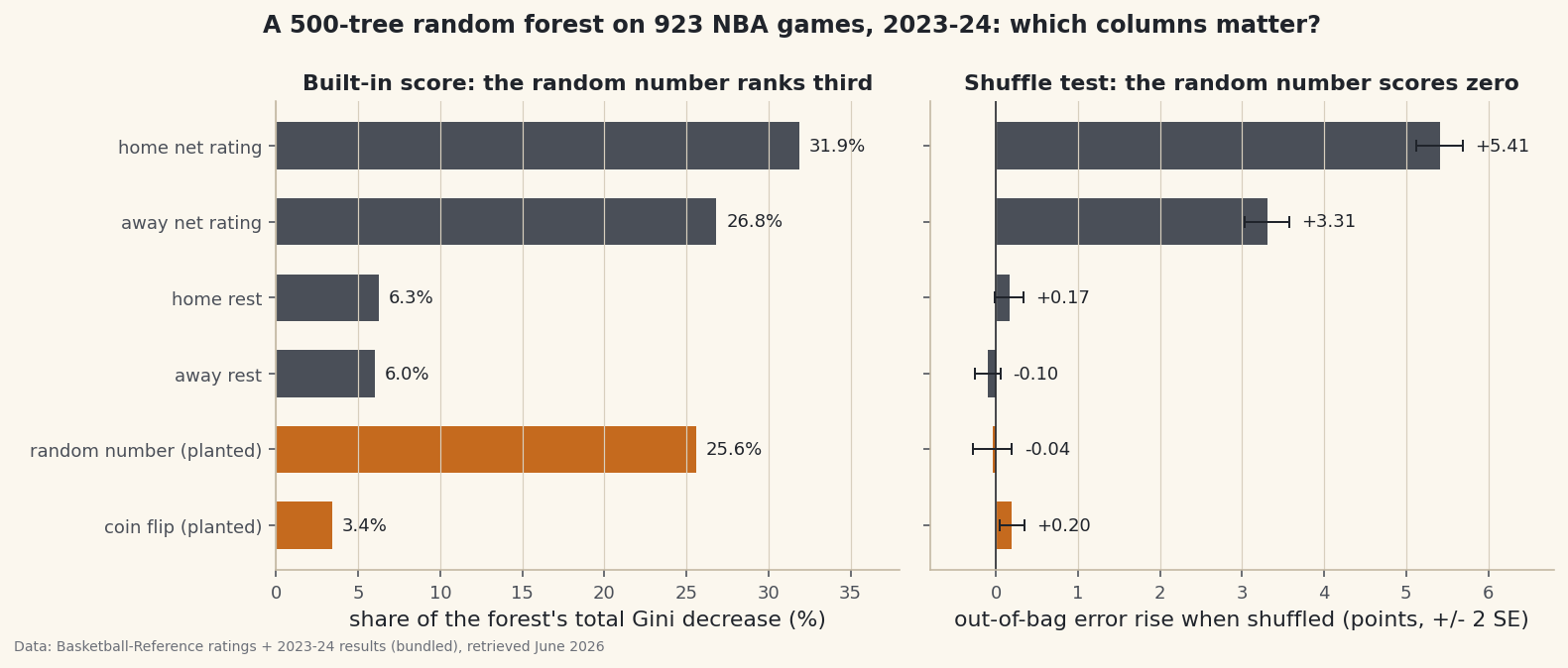
   Add up 107,274 such drops and the ranking is wrong at third place. The home net rating leads with 31.9% and the away net rating follows with 26.8%, but the random number is right behind at 25.6%, about four times either rest column (6.3% and 6.0%), and the trees split on it 28,082 times, 26.2% of all splits and more than on any column that means something. The coin, the other planted column, comes last at 3.4%. Both are pure noise; the difference between them is the number of values. Deep in a tree, where a node holds a handful of games, a column with 923 values can almost always find some cut that separates a few wins from a few losses by chance, and every such cut is credited to it as a real impurity drop. The coin can offer only one cut, so it is chosen far less often. The score measures how useful a column was for describing the training games, and a column that can single out any game is useful for that whether or not it means anything. Strobl, Boulesteix, Zeileis and Hothorn (2007) showed in simulations that random forest importance measures “are not reliable in situations where potential predictor variables vary in their scale of measurement or their number of categories,” and traced the bias to two places: how single trees choose their splits, and bootstrap sampling with replacement.

6. Shuffle a column and see what breaks

   The repair asks a different question: not how much a column was used, but how much the predictions depend on it. Breiman’s recipe: after a tree is grown, “the values of the mth variable in the out-of-bag examples are randomly permuted and the out-of-bag data is run down the corresponding tree.” Shuffling breaks the column’s link to the result while keeping its values, so a column the tree truly relies on costs accuracy when shuffled, and a column it merely used to memorise training games costs nothing on games it never saw. Breiman’s paper compares the forest’s out-of-bag votes before and after; on 923 games that version is noisy, so the code below records each tree’s rise in error and averages over the 500 trees, reporting a standard error with it.

   def permutation_importance(trees, in_bag, X, y, seed=7):
       """Breiman's recipe, tree by tree: shuffle one column on the games a tree never saw, run
       them down that tree again, and record how much its error rises. Average over the trees."""
       rng = np.random.default_rng(seed)
       rise = np.zeros((len(trees), X.shape[1]))
       for b, (t, o) in enumerate(zip(trees, ~in_bag)):
           rows = np.flatnonzero(o)
           Xo, yo = X[rows], y[rows]
           err = 1 - accuracy(predict(t, Xo), yo)
           for j in range(X.shape[1]):
               Xp = Xo.copy()
               Xp[:, j] = rng.permutation(Xp[:, j])           # noise up column j
               rise[b, j] = (1 - accuracy(predict(t, Xp), yo)) - err
       return rise.mean(0), rise.std(0, ddof=1) / np.sqrt(len(trees))
   
   rise, se = permutation_importance(trees, in_bag, X[tr], y[tr])
   print("rise in a tree's out-of-bag error when one column is shuffled, averaged over 500 trees:")
   for j in np.argsort(-rise):
       print(f"  {FEATURES[j]:10s} {100 * rise[j]:+6.2f} points   (+/- {200 * se[j]:.2f})")

   Shuffled one at a time: the net ratings matter, the random number does not

   rise in a tree's out-of-bag error when one column is shuffled, averaged over 500 trees:
     home_nrtg   +5.41 points   (+/- 0.28)
     away_nrtg   +3.31 points   (+/- 0.27)
     coin        +0.20 points   (+/- 0.15)
     home_rest   +0.17 points   (+/- 0.17)
     noise       -0.04 points   (+/- 0.24)
     away_rest   -0.10 points   (+/- 0.16)

   The ranking changes where it should. Shuffling the home net rating raises a tree’s out-of-bag error by 5.41 points and the away net rating by 3.31, each far outside its error bar. The random number, third on the built-in score, now scores −0.04 ± 0.24, which is zero: the trees used it constantly and none of them needed it. Neither rest column clears its error bar either: home rest at +0.17 ± 0.17 sits right on the edge and away rest is below zero, which fits the rest-days study’s finding of an effect that is “real, and small”, too small for 923 games to show this way. The shuffle score is not bias-free in general: Strobl and colleagues found it can favour many-valued columns too, through the trees it is computed on. Here it held.

   The coin is the warning in this table. A column of coin flips should score zero, and it scores +0.20 ± 0.15, an interval that misses zero. The ± treats the 500 trees as 500 independent experiments, and they are not: all of them were grown from the same 923 games and scored on overlapping out-of-bag sets, so their errors move together and the standard error is too small. The next step measures by how much.

7. Again, with fresh noise, and with a floor

   One forest and one draw of the planted columns could be a fluke. Five fresh draws, each with a fresh forest, test both findings, and a sixth forest tries a cheap fix for the built-in score: require at least 20 games in every leaf, as the decision tree did, so the trees cannot chase single games.

   print("five fresh noise columns, a fresh forest each time:")
   print("  draw   noise share   rank   shuffle rise, points: noise          coin")
   Xr = X[tr].copy()
   redraw = []
   for draw in range(1, 6):
       r = np.random.default_rng(1000 + draw)
       Xr[:, 4], Xr[:, 5] = r.random(len(tr)), r.integers(0, 2, len(tr))
       t_r, ib_r, lg_r = forest(Xr, y[tr], seed=draw)
       s_r = impurity_importance(lg_r, len(tr))
       s_r = s_r / s_r.sum()
       rise_r, se_r = permutation_importance(t_r, ib_r, Xr, y[tr], seed=draw)
       redraw.append((s_r[4], int((s_r > s_r[4]).sum()) + 1, rise_r[4], se_r[4], rise_r[5], se_r[5]))
       print(f"  {draw:4d}   {s_r[4]:11.1%}   {redraw[-1][1]:4d}   {100 * rise_r[4]:+21.2f} (+/- {200 * se_r[4]:.2f})"
             f"   {100 * rise_r[5]:+.2f} (+/- {200 * se_r[5]:.2f})")
   
   t20, _, lg20 = forest(X[tr], y[tr], min_leaf=20)
   s20 = impurity_importance(lg20, len(tr))
   s20 = s20 / s20.sum()
   print(f"with at least 20 games a leaf: noise share {s20[4]:.1%}, rank {int((s20 > s20[4]).sum()) + 1}; "
         f"held-out accuracy {accuracy(vote(t20, X[te]), y[te]):.1%}")

   Five more draws of noise, and a minimum leaf size

   five fresh noise columns, a fresh forest each time:
     draw   noise share   rank   shuffle rise, points: noise          coin
        1         25.2%      3                   -0.39 (+/- 0.23)   +0.10 (+/- 0.15)
        2         26.1%      3                   -0.05 (+/- 0.21)   +0.17 (+/- 0.15)
        3         26.0%      2                   -0.10 (+/- 0.22)   +0.09 (+/- 0.16)
        4         25.8%      3                   -0.04 (+/- 0.22)   +0.02 (+/- 0.17)
        5         26.3%      3                   +0.16 (+/- 0.23)   -0.03 (+/- 0.15)
   with at least 20 games a leaf: noise share 8.5%, rank 3; held-out accuracy 67.5%

   The built-in score is no fluke. In all five draws the random number takes between 25.2% and 26.3% of the total and ranks second or third, never below the rest columns. The shuffle score stays near zero, from −0.39 to +0.16 points, but those five values spread with a standard deviation of 0.20 points, 1.79 times the 0.11-point standard error the per-tree calculation reports on average. Counting the first run, 3 of the 12 intervals for the planted columns miss zero: the random number in draw 1, the coin in draw 2 and the coin in the first run. Intervals that worked as advertised would miss about once in twenty. So the shuffle score ranks the columns correctly every time, while its error bar needs the same treatment as any other small-sample claim: repeat the experiment, and widen the interval to the spread you see.

   The floor helps the built-in score without curing it. With at least 20 games a leaf, the random number’s share falls from 25.6% to 8.5%, because the small nodes where it did its damage are gone, but it still ranks third, above both rest columns. The same floor lifts the held-out accuracy to 67.5%, 208 games, inside the ±5.3-point margin of the 202 the fully grown forest called, so this test set cannot say the floor is better.

8. Draw both rankings

   The chart puts the two scores side by side, the planted columns in orange. The left panel is what a forest reports by default; the right panel is what shuffling shows.

   import matplotlib.pyplot as plt
   
   LABELS = ["home net rating", "away net rating", "home rest", "away rest", "random number (planted)", "coin flip (planted)"]
   REAL, PLANTED = "#4A4F58", "#C56A1E"
   colors = [PLANTED if j >= 4 else REAL for j in range(len(FEATURES))]
   order = np.arange(len(FEATURES))[::-1]                       # first feature at the top
   fig, (ax1, ax2) = plt.subplots(1, 2, figsize=(11, 4.6), sharey=True)
   ax1.barh(order, 100 * share, color=colors, height=0.62)
   for j in range(len(FEATURES)):
       ax1.text(100 * share[j] + 0.6, order[j], f"{share[j]:.1%}", va="center", fontsize=9)
   ax1.set_yticks(order)
   ax1.set_yticklabels(LABELS)
   ax1.set_xlim(0, 38)
   ax1.set_xlabel("share of the forest's total Gini decrease (%)")
   ax1.set_title("Built-in score: the random number ranks third", fontsize=11)
   ax1.grid(axis="x")
   ax1.grid(axis="y", visible=False)
   ax2.barh(order, 100 * rise, xerr=200 * se, color=colors, height=0.62, error_kw={"ecolor": "#20242B", "capsize": 3, "lw": 1})
   for j in range(len(FEATURES)):
       x = max(100 * rise[j] + 200 * se[j], 0) + 0.15
       ax2.text(x, order[j], f"{100 * rise[j]:+.2f}", va="center", fontsize=9)
   ax2.axvline(0, color="#20242B", lw=0.8)
   ax2.set_xlim(-0.8, 6.8)
   ax2.set_xlabel("out-of-bag error rise when shuffled (points, +/- 2 SE)")
   ax2.set_title("Shuffle test: the random number scores zero", fontsize=11)
   ax2.grid(axis="x")
   ax2.grid(axis="y", visible=False)
   fig.suptitle("A 500-tree random forest on 923 NBA games, 2023-24: which columns matter?", fontsize=12, fontweight="bold")
   fig.tight_layout()
   fig.savefig("importance_two_ways.png", dpi=144)

   

   Read across a row and the problem is plain. The random number’s orange bar on the left is almost as long as the away net rating’s; on the right it has vanished, while the two net ratings keep long bars on both sides. Whenever a forest’s columns differ in how many values they take, as real data almost always does, a ranking from the left panel will flatter the columns with many values, so check it against the right one before telling anyone what matters.

Where this breaks

Six limits. The problem leaks. The two net ratings summarise the whole 2023-24 season, including the games being predicted, as in the decision tree and the rest of this course; the accuracies teach the method and are not a forecast of anything. 308 games decide little. The ±5.3-point margin on held-out accuracy swallows every comparison between the tree, the forests and the floor; to compare models, use the k-fold cross-validation tutorial’s repeated splits. The shuffle score’s error bar is too narrow. Its trees share their data, so the per-tree standard error understated the spread across fresh runs by a factor of 1.79 here; treat a single run’s interval as a lower bound, and when many columns are screened at once, the multiple-comparisons correction applies too. Shuffling has its own blind spot. When two columns carry the same information, shuffling one costs little because the trees fall back on the other, so a shuffle score can understate both; the two net ratings here are not copies, but a forest given ORtg, DRtg and net rating together could show it. The planted columns are an extreme. Real columns with many values, a date, an ID, a minutes total, carry some signal and some room to memorise, and nothing tells you the mix; the planted pair only shows that the built-in score cannot separate the two. One season, one problem, one forest design. Two columns per split, fully grown trees and 500 of them are common choices, not the only ones, and another season, sport or target would move every number on this page; the method, not the figures, is what carries over.

Sources. Games and ratings: Basketball-Reference’s 2023-24 schedule pages (leagues/NBA_2024_games-*.html) and team ratings page (leagues/NBA_2024_ratings.html), read with pandas by build/make_nba_samples.py and bundled in June 2026 as nba_home_results.csv (1,231 games, the In-Season Tournament final included) and nba_ratings.csv. Bagging: L. Breiman, “Bagging Predictors,” Machine Learning 24(2), 1996, pp. 123-140, doi:10.1007/BF00058655; the sentence quoted is from the abstract of its 1994 Berkeley technical report (No. 421), read on 14 October 2026. Random forests: L. Breiman, “Random Forests,” Machine Learning 45(1), 2001, pp. 5-32, doi:10.1023/A:1010933404324, quoted from the author’s January 2001 copy, read on 14 October 2026. Random subspaces: T. K. Ho, “The Random Subspace Method for Constructing Decision Forests,” IEEE Transactions on Pattern Analysis and Machine Intelligence 20(8), 1998, pp. 832-844, doi:10.1109/34.709601. Importance bias: C. Strobl, A.-L. Boulesteix, A. Zeileis and T. Hothorn, “Bias in Random Forest Variable Importance Measures: Illustrations, Sources and a Solution,” BMC Bioinformatics 8, 2007, article 25, doi:10.1186/1471-2105-8-25, whose proposed fix uses a different tree algorithm and subsampling without replacement, not shown here. The bootstrap: B. Efron, “Bootstrap Methods: Another Look at the Jackknife,” Annals of Statistics 7(1), 1979, doi:10.1214/aos/1176344552. Every number on this page is recomputed by the tutorial’s script, whose asserts fail rather than print a figure they cannot reproduce.

Troubleshooting